CoxPHFitter
- class lifelines.fitters.coxph_fitter.CoxPHFitter(baseline_estimation_method: str = 'breslow', penalizer: float | ndarray = 0.0, strata: List[str] | str | None = None, l1_ratio: float = 0.0, n_baseline_knots: int | None = None, knots: List | None = None, breakpoints: List | None = None, **kwargs)
This class implements fitting Cox’s proportional hazard model.
\[h(t|x) = h_0(t) \exp((x - \overline{x})' \beta)\]The baseline hazard, \(h_0(t)\) can be modeled in two ways:
1. (default) non-parametrically, using Breslow’s method. In this case, the entire model is the traditional semi-parametric Cox model. Ties are handled using Efron’s method.
parametrically, using a pre-specified number of cubic splines, or piecewise values.
This is specified using the
baseline_estimation_methodparameter in the initialization (default ="breslow")- Parameters:
alpha (float, optional (default=0.05)) – the level in the confidence intervals.
baseline_estimation_method (string, optional) – specify how the fitter should estimate the baseline.
"breslow","spline", or"piecewise"penalizer (float or array, optional (default=0.0)) – Attach a penalty to the size of the coefficients during regression. This improves stability of the estimates and controls for high correlation between covariates. For example, this shrinks the magnitude value of \(\beta_i\). See
l1_ratiobelow. The penalty term is \(\text{penalizer} \left( \frac{1-\text{l1_ratio}}{2} ||\beta||_2^2 + \text{l1_ratio}||\beta||_1\right)\).Alternatively, penalizer is an array equal in size to the number of parameters, with penalty coefficients for specific variables. For example, penalizer=0.01 * np.ones(p) is the same as penalizer=0.01
l1_ratio (float, optional (default=0.0)) – Specify what ratio to assign to a L1 vs L2 penalty. Same as scikit-learn. See
penalizerabove.strata (list, optional) – specify a list of columns to use in stratification. This is useful if a categorical covariate does not obey the proportional hazard assumption. This is used similar to the strata expression in R. See http://courses.washington.edu/b515/l17.pdf.
n_baseline_knots (int) – Used when
baseline_estimation_method="spline". Set the number of knots (interior & exterior) in the baseline hazard, which will be placed evenly along the time axis. Should be at least 2. Royston et. al, the authors of this model, suggest 4 to start, but any values between 2 and 8 are reasonable. If you need to customize the timestamps used to calculate the curve, use theknotsparameter instead.knots (list, optional) – When
baseline_estimation_method="spline", this allows customizing the points in the time axis for the baseline hazard curve. To use evenly-spaced points in time, then_baseline_knotsparameter can be employed instead.breakpoints (list, optional) – Used when
baseline_estimation_method="piecewise". Set the positions of the baseline hazard breakpoints.
Examples
from lifelines.datasets import load_rossi
from lifelines import CoxPHFitter
rossi = load_rossi()
cph = CoxPHFitter()
cph.fit(rossi, 'week', 'arrest')
cph.print_summary()
- params_
The estimated coefficients. Changed in version 0.22.0: use to be
.hazards_- Type:
Series
- hazard_ratios_
The exp(coefficients)
- Type:
Series
- confidence_intervals_
The lower and upper confidence intervals for the hazard coefficients
- Type:
DataFrame
- durations
The durations provided
- Type:
Series
- event_observed
The event_observed variable provided
- Type:
Series
- weights
The event_observed variable provided
- Type:
Series
- variance_matrix_
The variance matrix of the coefficients
- Type:
DataFrame
- strata
the strata provided
- Type:
list
- standard_errors_
the standard errors of the estimates
- Type:
Series
- log_likelihood_
the log-likelihood at the fitted coefficients
- Type:
float
- AIC_
the AIC at the fitted coefficients (if using splines for baseline hazard)
- Type:
float
- partial_AIC_
the AIC at the fitted coefficients (if using non-parametric inference for baseline hazard)
- Type:
float
- baseline_hazard_
the baseline hazard evaluated at the observed times. Estimated using Breslow’s method.
- Type:
DataFrame
- baseline_cumulative_hazard_
the baseline cumulative hazard evaluated at the observed times. Estimated using Breslow’s method.
- Type:
DataFrame
- baseline_survival_
the baseline survival evaluated at the observed times. Estimated using Breslow’s method.
- Type:
DataFrame
- summary
a Dataframe of the coefficients, p-values, CIs, etc. found in
print_summary- Type:
Dataframe
- plot_covariate_groups()
see
plot_covariate_groups()
- plot_partial_effects_on_outcome()
see
plot_partial_effects_on_outcome()
- predict_median()
see
predict_median()
- predict_expectation()
- predict_percentile()
- predict_survival_function()
- predict_partial_hazard()
- predict_log_partial_hazard()
- predict_cumulative_hazard()
- log_likelihood_ratio_test()
- compute_followup_hazard_ratios(training_df: DataFrame, followup_times: Iterable) DataFrame
Recompute the hazard ratio at different follow-up times (lifelines handles accounting for updated censoring and updated durations). This is useful because we need to remember that the hazard ratio is actually a weighted-average of period-specific hazard ratios.
- Parameters:
training_df (pd.DataFrame) – The same dataframe used to train the model
followup_times (Iterable) – a list/array of follow-up times to recompute the hazard ratio at.
- fit(df: DataFrame, duration_col: str | None = None, event_col: str | None = None, show_progress: bool = False, initial_point: ndarray | None = None, strata: List[str] | str | None = None, weights_col: str | None = None, cluster_col: str | None = None, robust: bool = False, batch_mode: bool | None = None, timeline: Iterator | None = None, formula: str = None, entry_col: str = None, fit_options: dict | None = None) CoxPHFitter
Fit the Cox proportional hazard model to a right-censored dataset. Alias of fit_right_censoring.
- Parameters:
df (DataFrame) – a Pandas DataFrame with necessary columns duration_col and event_col (see below), covariates columns, and special columns (weights, strata). duration_col refers to the lifetimes of the subjects. event_col refers to whether the ‘death’ events was observed: 1 if observed, 0 else (censored).
duration_col (string) – the name of the column in DataFrame that contains the subjects’ lifetimes.
event_col (string, optional) – the name of the column in DataFrame that contains the subjects’ death observation. If left as None, assume all individuals are uncensored.
weights_col (string, optional) – an optional column in the DataFrame, df, that denotes the weight per subject. This column is expelled and not used as a covariate, but as a weight in the final regression. Default weight is 1. This can be used for case-weights. For example, a weight of 2 means there were two subjects with identical observations. This can be used for sampling weights. In that case, use
robust=Trueto get more accurate standard errors.cluster_col (string, optional) – specifies what column has unique identifiers for clustering covariances. Using this forces the sandwich estimator (robust variance estimator) to be used.
entry_col (str, optional) – a column denoting when a subject entered the study, i.e. left-truncation.
strata (list or string, optional) – specify a column or list of columns n to use in stratification. This is useful if a categorical covariate does not obey the proportional hazard assumption. This is used similar to the
strataexpression in R. See http://courses.washington.edu/b515/l17.pdf.robust (bool, optional (default=False)) – Compute the robust errors using the Huber sandwich estimator, aka Wei-Lin estimate. This does not handle ties, so if there are high number of ties, results may significantly differ. See “The Robust Inference for the Cox Proportional Hazards Model”, Journal of the American Statistical Association, Vol. 84, No. 408 (Dec., 1989), pp. 1074- 1078
formula (str, optional) – an Wilkinson formula, like in R and statsmodels, for the right-hand-side. If left as None, all columns not assigned as durations, weights, etc. are used. Uses the library Formulaic for parsing.
batch_mode (bool, optional) – enabling batch_mode can be faster for datasets with a large number of ties. If left as None, lifelines will choose the best option.
show_progress (bool, optional (default=False)) – since the fitter is iterative, show convergence diagnostics. Useful if convergence is failing.
initial_point ((d,) numpy array, optional) – initialize the starting point of the iterative algorithm. Default is the zero vector.
fit_options (dict, optional) – pass kwargs for the fitting algorithm. For semi-parametric models, this is the Newton-Raphson method (see method _newton_raphson_for_efron_model for kwargs)
- Returns:
self – self with additional new properties:
print_summary,hazards_,confidence_intervals_,baseline_survival_, etc.- Return type:
Examples
from lifelines import CoxPHFitter

df = pd.DataFrame({
    'T': [5, 3, 9, 8, 7, 4, 4, 3, 2, 5, 6, 7],
    'E': [1, 1, 1, 1, 1, 1, 0, 0, 1, 1, 1, 0],
    'var': [0, 0, 0, 0, 1, 1, 1, 1, 1, 2, 2, 2],
    'age': [4, 3, 9, 8, 7, 4, 4, 3, 2, 5, 6, 7],
})

cph = CoxPHFitter()
cph.fit(df, 'T', 'E')
cph.print_summary()
cph.predict_median(df)
from lifelines import CoxPHFitter

df = pd.DataFrame({
    'T': [5, 3, 9, 8, 7, 4, 4, 3, 2, 5, 6, 7],
    'E': [1, 1, 1, 1, 1, 1, 0, 0, 1, 1, 1, 0],
    'var': [0, 0, 0, 0, 1, 1, 1, 1, 1, 2, 2, 2],
    'weights': [1.1, 0.5, 2.0, 1.6, 1.2, 4.3, 1.4, 4.5, 3.0, 3.2, 0.4, 6.2],
    'month': [10, 3, 9, 8, 7, 4, 4, 3, 2, 5, 6, 7],
    'age': [4, 3, 9, 8, 7, 4, 4, 3, 2, 5, 6, 7],
})

cph = CoxPHFitter()
cph.fit(df, 'T', 'E', strata=['month', 'age'], robust=True, weights_col='weights')
cph.print_summary()
- fit_interval_censoring(df: DataFrame, lower_bound_col: str, upper_bound_col: str, event_col: str | None = None, show_progress: bool = False, initial_point: ndarray | None = None, strata: List[str] | str | None = None, weights_col: str | None = None, cluster_col: str | None = None, robust: bool = False, batch_mode: bool | None = None, timeline: Iterator | None = None, formula: str = None, entry_col: str = None, fit_options: dict | None = None) CoxPHFitter
Fit the Cox proportional hazard model to an interval censored dataset.
- Parameters:
df (DataFrame) – a Pandas DataFrame with necessary columns duration_col and event_col (see below), covariates columns, and special columns (weights, strata). duration_col refers to the lifetimes of the subjects. event_col refers to whether the ‘death’ events was observed: 1 if observed, 0 else (censored).
lower_bound_col (string) – the name of the column in DataFrame that contains the lower bounds of the intervals.
upper_bound_col (string) – the name of the column in DataFrame that contains the upper bounds of the intervals.
event_col (string, optional) – the name of the column in DataFrame that contains the subjects’ death observation. If left as None, this is inferred based on the upper and lower interval limits (equal implies observed death.)
weights_col (string, optional) – an optional column in the DataFrame, df, that denotes the weight per subject. This column is expelled and not used as a covariate, but as a weight in the final regression. Default weight is 1. This can be used for case-weights. For example, a weight of 2 means there were two subjects with identical observations. This can be used for sampling weights. In that case, use
robust=Trueto get more accurate standard errors.cluster_col (string, optional) – specifies what column has unique identifiers for clustering covariances. Using this forces the sandwich estimator (robust variance estimator) to be used.
entry_col (str, optional) – a column denoting when a subject entered the study, i.e. left-truncation.
strata (list or string, optional) – specify a column or list of columns n to use in stratification. This is useful if a categorical covariate does not obey the proportional hazard assumption. This is used similar to the
strataexpression in R. See http://courses.washington.edu/b515/l17.pdf.robust (bool, optional (default=False)) – Compute the robust errors using the Huber sandwich estimator, aka Wei-Lin estimate. This does not handle ties, so if there are high number of ties, results may significantly differ. See “The Robust Inference for the Cox Proportional Hazards Model”, Journal of the American Statistical Association, Vol. 84, No. 408 (Dec., 1989), pp. 1074- 1078
formula (str, optional) – an Wilkinson formula, like in R and statsmodels, for the right-hand-side. If left as None, all columns not assigned as durations, weights, etc. are used.
batch_mode (bool, optional) – enabling batch_mode can be faster for datasets with a large number of ties. If left as None, lifelines will choose the best option.
show_progress (bool, optional (default=False)) – since the fitter is iterative, show convergence diagnostics. Useful if convergence is failing.
initial_point ((d,) numpy array, optional) – initialize the starting point of the iterative algorithm. Default is the zero vector.
- Returns:
self – self with additional new properties:
print_summary,hazards_,confidence_intervals_,baseline_survival_, etc.- Return type:
Examples
from lifelines import CoxPHFitter

df = pd.DataFrame({
    'T': [5, 3, 9, 8, 7, 4, 4, 3, 2, 5, 6, 7],
    'E': [1, 1, 1, 1, 1, 1, 0, 0, 1, 1, 1, 0],
    'var': [0, 0, 0, 0, 1, 1, 1, 1, 1, 2, 2, 2],
    'age': [4, 3, 9, 8, 7, 4, 4, 3, 2, 5, 6, 7],
})

cph = CoxPHFitter()
cph.fit(df, 'T', 'E')
cph.print_summary()
cph.predict_median(df)
from lifelines import CoxPHFitter

df = pd.DataFrame({
    'T': [5, 3, 9, 8, 7, 4, 4, 3, 2, 5, 6, 7],
    'E': [1, 1, 1, 1, 1, 1, 0, 0, 1, 1, 1, 0],
    'var': [0, 0, 0, 0, 1, 1, 1, 1, 1, 2, 2, 2],
    'weights': [1.1, 0.5, 2.0, 1.6, 1.2, 4.3, 1.4, 4.5, 3.0, 3.2, 0.4, 6.2],
    'month': [10, 3, 9, 8, 7, 4, 4, 3, 2, 5, 6, 7],
    'age': [4, 3, 9, 8, 7, 4, 4, 3, 2, 5, 6, 7],
})

cph = CoxPHFitter()
cph.fit(df, 'T', 'E', strata=['month', 'age'], robust=True, weights_col='weights')
cph.print_summary()
- fit_left_censoring(df: DataFrame, duration_col: str | None = None, event_col: str | None = None, show_progress: bool = False, initial_point: ndarray | None = None, strata: List[str] | str | None = None, weights_col: str | None = None, cluster_col: str | None = None, robust: bool = False, batch_mode: bool | None = None, timeline: Iterator | None = None, formula: str = None, entry_col: str = None, fit_options: dict | None = None) CoxPHFitter
Fit the Cox proportional hazard model to a left censored dataset.
- Parameters:
df (DataFrame) – a Pandas DataFrame with necessary columns duration_col and event_col (see below), covariates columns, and special columns (weights, strata). duration_col refers to the lifetimes of the subjects. event_col refers to whether the ‘death’ events was observed: 1 if observed, 0 else (censored).
duration_col (string) – the name of the column in DataFrame that contains the subjects’ lifetimes.
event_col (string, optional) – the name of the column in DataFrame that contains the subjects’ death observation. If left as None, assume all individuals are uncensored.
weights_col (string, optional) – an optional column in the DataFrame, df, that denotes the weight per subject. This column is expelled and not used as a covariate, but as a weight in the final regression. Default weight is 1. This can be used for case-weights. For example, a weight of 2 means there were two subjects with identical observations. This can be used for sampling weights. In that case, use
robust=Trueto get more accurate standard errors.cluster_col (string, optional) – specifies what column has unique identifiers for clustering covariances. Using this forces the sandwich estimator (robust variance estimator) to be used.
entry_col (str, optional) – a column denoting when a subject entered the study, i.e. left-truncation.
strata (list or string, optional) – specify a column or list of columns n to use in stratification. This is useful if a categorical covariate does not obey the proportional hazard assumption. This is used similar to the
strataexpression in R. See http://courses.washington.edu/b515/l17.pdf.robust (bool, optional (default=False)) – Compute the robust errors using the Huber sandwich estimator, aka Wei-Lin estimate. This does not handle ties, so if there are high number of ties, results may significantly differ. See “The Robust Inference for the Cox Proportional Hazards Model”, Journal of the American Statistical Association, Vol. 84, No. 408 (Dec., 1989), pp. 1074- 1078
formula (str, optional) – an Wilkinson formula, like in R and statsmodels, for the right-hand-side. If left as None, all columns not assigned as durations, weights, etc. are used.
batch_mode (bool, optional) – enabling batch_mode can be faster for datasets with a large number of ties. If left as None, lifelines will choose the best option.
show_progress (bool, optional (default=False)) – since the fitter is iterative, show convergence diagnostics. Useful if convergence is failing.
initial_point ((d,) numpy array, optional) – initialize the starting point of the iterative algorithm. Default is the zero vector.
- Returns:
self – self with additional new properties:
print_summary,hazards_,confidence_intervals_,baseline_survival_, etc.- Return type:
Examples
from lifelines import CoxPHFitter

df = pd.DataFrame({
    'T': [5, 3, 9, 8, 7, 4, 4, 3, 2, 5, 6, 7],
    'E': [1, 1, 1, 1, 1, 1, 0, 0, 1, 1, 1, 0],
    'var': [0, 0, 0, 0, 1, 1, 1, 1, 1, 2, 2, 2],
    'age': [4, 3, 9, 8, 7, 4, 4, 3, 2, 5, 6, 7],
})

cph = CoxPHFitter()
cph.fit(df, 'T', 'E')
cph.print_summary()
cph.predict_median(df)
from lifelines import CoxPHFitter

df = pd.DataFrame({
    'T': [5, 3, 9, 8, 7, 4, 4, 3, 2, 5, 6, 7],
    'E': [1, 1, 1, 1, 1, 1, 0, 0, 1, 1, 1, 0],
    'var': [0, 0, 0, 0, 1, 1, 1, 1, 1, 2, 2, 2],
    'weights': [1.1, 0.5, 2.0, 1.6, 1.2, 4.3, 1.4, 4.5, 3.0, 3.2, 0.4, 6.2],
    'month': [10, 3, 9, 8, 7, 4, 4, 3, 2, 5, 6, 7],
    'age': [4, 3, 9, 8, 7, 4, 4, 3, 2, 5, 6, 7],
})

cph = CoxPHFitter()
cph.fit(df, 'T', 'E', strata=['month', 'age'], robust=True, weights_col='weights')
cph.print_summary()
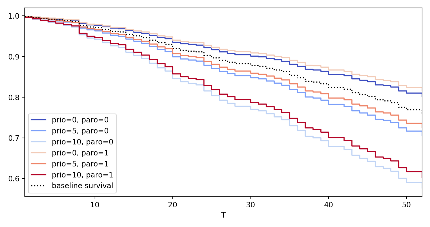
- plot_partial_effects_on_outcome(covariates, values, plot_baseline=True, y='survival_function', **kwargs)
Produces a plot comparing the baseline curve of the model versus what happens when a covariate(s) is varied over values in a group. This is useful to compare subjects’ survival as we vary covariate(s), all else being held equal.
The baseline curve is equal to the predicted curve at all average values (median for ordinal, and mode for categorical) in the original dataset. This same logic is applied to the stratified datasets if
stratawas used in fitting.- Parameters:
covariates (string or list) – a string (or list of strings) of the covariate(s) in the original dataset that we wish to vary.
values (1d or 2d iterable) – an iterable of the specific values we wish the covariate(s) to take on.
plot_baseline (bool) – also display the baseline survival, defined as the survival at the mean of the original dataset.
y (str) – one of “survival_function”, or “cumulative_hazard”
kwargs – pass in additional plotting commands.
- Returns:
ax – the matplotlib axis that be edited.
- Return type:
matplotlib axis, or list of axis’
Examples
from lifelines import datasets, CoxPHFitter
rossi = datasets.load_rossi()

cph = CoxPHFitter().fit(rossi, 'week', 'arrest')
cph.plot_partial_effects_on_outcome('prio', values=arange(0, 15, 3), cmap='coolwarm')
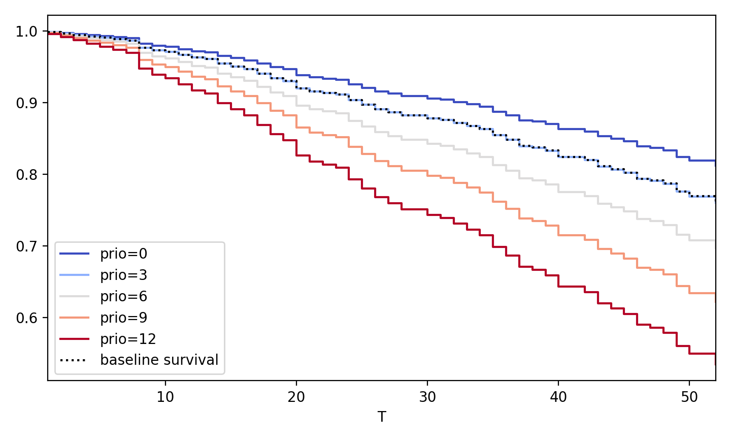
# multiple variables at once
cph.plot_partial_effects_on_outcome(['prio', 'paro'], values=[
 [0,  0],
 [5,  0],
 [10, 0],
 [0,  1],
 [5,  1],
 [10, 1]
], cmap='coolwarm')
# if you have categorical variables, you can do the following to see the
# effect of all the categories on one plot.
cph.plot_partial_effects_on_outcome('categorical_var', values=["A", "B", "C"])
- print_summary(decimals=2, style=None, columns=None, **kwargs)
Print summary statistics describing the fit, the coefficients, and the error bounds.
- Parameters:
decimals (int, optional (default=2)) – specify the number of decimal places to show
style (string) – {html, ascii, latex}
columns – only display a subset of
summarycolumns. Default all.kwargs – print additional metadata in the output (useful to provide model names, dataset names, etc.) when comparing multiple outputs.
- class lifelines.fitters.coxph_fitter.SemiParametricPHFitter(penalizer: float | ndarray = 0.0, strata: List[str] | str | None = None, l1_ratio: float = 0.0, **kwargs)
This class implements fitting Cox’s proportional hazard model using Efron’s method for ties.
\[h(t|x) = h_0(t) \exp((x - \overline{x})' \beta)\]The baseline hazard, \(h_0(t)\) is modeled non-parametrically (using Breslow’s method).
Note
This is a “hidden” class that is invoked when using
baseline_estimation_method="breslow"(the default). You probably want to useCoxPHFitter, not this.- Parameters:
alpha (float, optional (default=0.05)) – the level in the confidence intervals.
penalizer (float or array, optional (default=0.0)) – Attach a penalty to the size of the coefficients during regression. This improves stability of the estimates and controls for high correlation between covariates. For example, this shrinks the magnitude value of \(\beta_i\). See
l1_ratiobelow. The penalty term is \(\text{penalizer} \left( \frac{1-\text{l1_ratio}}{2} ||\beta||_2^2 + \text{l1_ratio}||\beta||_1\right)\).Alternatively, penalizer is an array equal in size to the number of parameters, with penalty coefficients for specific variables. For example, penalizer=0.01 * np.ones(p) is the same as penalizer=0.01
l1_ratio (float, optional (default=0.0)) – Specify what ratio to assign to a L1 vs L2 penalty. Same as scikit-learn. See
penalizerabove.strata (list, optional) – specify a list of columns to use in stratification. This is useful if a categorical covariate does not obey the proportional hazard assumption. This is used similar to the strata expression in R. See http://courses.washington.edu/b515/l17.pdf.
Examples
from lifelines.datasets import load_rossi
from lifelines import CoxPHFitter
rossi = load_rossi()
cph = CoxPHFitter()
cph.fit(rossi, 'week', 'arrest')
cph.print_summary()
- params_
The estimated coefficients. Changed in version 0.22.0: use to be
.hazards_- Type:
Series
- hazard_ratios_
The exp(coefficients)
- Type:
Series
- confidence_intervals_
The lower and upper confidence intervals for the hazard coefficients
- Type:
DataFrame
- durations
The durations provided
- Type:
Series
- event_observed
The event_observed variable provided
- Type:
Series
- weights
The event_observed variable provided
- Type:
Series
- variance_matrix_
The variance matrix of the coefficients
- Type:
DataFrame
- strata
the strata provided
- Type:
list
- standard_errors_
the standard errors of the estimates
- Type:
Series
- baseline_hazard_
- Type:
DataFrame
- baseline_cumulative_hazard_
- Type:
DataFrame
- baseline_survival_
- Type:
DataFrame
- property concordance_index_: float
The concordance score (also known as the c-index) of the fit. The c-index is a generalization of the ROC AUC to survival data, including censoring.
For this purpose, the
concordance_index_is a measure of the predictive accuracy of the fitted model onto the training dataset.References
- fit(df: DataFrame, duration_col: str | None = None, event_col: str | None = None, show_progress: bool = False, initial_point: ndarray | None = None, strata: List[str] | str | None = None, weights_col: str | None = None, cluster_col: str | None = None, robust: bool = False, batch_mode: bool | None = None, timeline: Iterator | None = None, formula: str = None, entry_col: str = None, fit_options: dict | None = None) SemiParametricPHFitter
Fit the Cox proportional hazard model to a dataset.
- Parameters:
df (DataFrame) – a Pandas DataFrame with necessary columns duration_col and event_col (see below), covariates columns, and special columns (weights, strata). duration_col refers to the lifetimes of the subjects. event_col refers to whether the ‘death’ events was observed: 1 if observed, 0 else (censored).
duration_col (string) – the name of the column in DataFrame that contains the subjects’ lifetimes.
event_col (string, optional) – the name of the column in DataFrame that contains the subjects’ death observation. If left as None, assume all individuals are uncensored.
weights_col (string, optional) – an optional column in the DataFrame, df, that denotes the weight per subject. This column is expelled and not used as a covariate, but as a weight in the final regression. Default weight is 1. This can be used for case-weights. For example, a weight of 2 means there were two subjects with identical observations. This can be used for sampling weights. In that case, use
robust=Trueto get more accurate standard errors.show_progress (bool, optional (default=False)) – since the fitter is iterative, show convergence diagnostics. Useful if convergence is failing.
initial_point ((d,) numpy array, optional) – initialize the starting point of the iterative algorithm. Default is the zero vector.
strata (list or string, optional) – specify a column or list of columns n to use in stratification. This is useful if a categorical covariate does not obey the proportional hazard assumption. This is used similar to the
strataexpression in R. See http://courses.washington.edu/b515/l17.pdf.robust (bool, optional (default=False)) – Compute the robust errors using the Huber sandwich estimator, aka Wei-Lin estimate. This does not handle ties, so if there are high number of ties, results may significantly differ. See “The Robust Inference for the Cox Proportional Hazards Model”, Journal of the American Statistical Association, Vol. 84, No. 408 (Dec., 1989), pp. 1074- 1078
cluster_col (string, optional) – specifies what column has unique identifiers for clustering covariances. Using this forces the sandwich estimator (robust variance estimator) to be used.
batch_mode (bool, optional) – enabling batch_mode can be faster for datasets with a large number of ties. If left as None, lifelines will choose the best option.
fit_options (dict, optional) –
- Override the default values in NR algorithm:
step_size: 0.95, precision: 1e-07, max_steps: 500,
- Returns:
self – self with additional new properties:
print_summary,hazards_,confidence_intervals_,baseline_survival_, etc.- Return type:
Note
Tied survival times are handled using Efron’s tie-method.
Examples
from lifelines import CoxPHFitter

df = pd.DataFrame({
    'T': [5, 3, 9, 8, 7, 4, 4, 3, 2, 5, 6, 7],
    'E': [1, 1, 1, 1, 1, 1, 0, 0, 1, 1, 1, 0],
    'var': [0, 0, 0, 0, 1, 1, 1, 1, 1, 2, 2, 2],
    'age': [4, 3, 9, 8, 7, 4, 4, 3, 2, 5, 6, 7],
})

cph = CoxPHFitter()
cph.fit(df, 'T', 'E')
cph.print_summary()
cph.predict_median(df)
from lifelines import CoxPHFitter

df = pd.DataFrame({
    'T': [5, 3, 9, 8, 7, 4, 4, 3, 2, 5, 6, 7],
    'E': [1, 1, 1, 1, 1, 1, 0, 0, 1, 1, 1, 0],
    'var': [0, 0, 0, 0, 1, 1, 1, 1, 1, 2, 2, 2],
    'weights': [1.1, 0.5, 2.0, 1.6, 1.2, 4.3, 1.4, 4.5, 3.0, 3.2, 0.4, 6.2],
    'month': [10, 3, 9, 8, 7, 4, 4, 3, 2, 5, 6, 7],
    'age': [4, 3, 9, 8, 7, 4, 4, 3, 2, 5, 6, 7],
})

cph = CoxPHFitter()
cph.fit(df, 'T', 'E', strata=['month', 'age'], robust=True, weights_col='weights')
cph.print_summary()
cph.predict_median(df)
- log_likelihood_ratio_test() StatisticalResult
This function computes the likelihood ratio test for the Cox model. We compare the existing model (with all the covariates) to the trivial model of no covariates.
- plot(columns=None, hazard_ratios=False, ax=None, **errorbar_kwargs)
Produces a visual representation of the coefficients (i.e. log hazard ratios), including their standard errors and magnitudes.
- Parameters:
columns (list, optional) – specify a subset of the columns to plot
hazard_ratios (bool, optional) – by default,
plotwill present the log-hazard ratios (the coefficients). However, by turning this flag to True, the hazard ratios are presented instead.errorbar_kwargs – pass in additional plotting commands to matplotlib errorbar command
Examples
from lifelines import datasets, CoxPHFitter
rossi = datasets.load_rossi()
cph = CoxPHFitter().fit(rossi, 'week', 'arrest')
cph.plot(hazard_ratios=True)
- Returns:
ax – the matplotlib axis that be edited.
- Return type:
matplotlib axis
- predict_cumulative_hazard(X: Series | DataFrame, times: ndarray | List[float] | None = None, conditional_after: List[int] | None = None) DataFrame
- Parameters:
X (numpy array or DataFrame) – a (n,d) covariate numpy array or DataFrame. If a DataFrame, columns can be in any order. If a numpy array, columns must be in the same order as the training data.
times (iterable, optional) – an iterable of increasing times to predict the cumulative hazard at. Default is the set of all durations (observed and unobserved). Uses a linear interpolation if points in time are not in the index.
conditional_after (iterable, optional) – Must be equal is size to X.shape[0] (denoted
nabove). An iterable (array, list, series) of possibly non-zero values that represent how long the subject has already lived for. Ex: if \(T\) is the unknown event time, then this represents \(s\) in \(T | T > s\). This is useful for knowing the remaining hazard/survival of censored subjects. The new timeline is the remaining duration of the subject, i.e. reset back to starting at 0.
- predict_expectation(X: DataFrame, conditional_after: ndarray | None = None) Series
Compute the expected lifetime, \(E[T]\), using covariates X. This algorithm to compute the expectation is to use the fact that \(E[T] = \int_0^\inf P(T > t) dt = \int_0^\inf S(t) dt\). To compute the integral, we use the trapezoidal rule to approximate the integral.
Caution
If the survival function doesn’t converge to 0, then the expectation is really infinity and the returned values are meaningless/too large. In that case, using
predict_medianorpredict_percentilewould be better.- Parameters:
X (numpy array or DataFrame) – a (n,d) covariate numpy array or DataFrame. If a DataFrame, columns can be in any order. If a numpy array, columns must be in the same order as the training data.
conditional_after (iterable, optional) – Must be equal is size to X.shape[0] (denoted n above). An iterable (array, list, series) of possibly non-zero values that represent how long the subject has already lived for. Ex: if \(T\) is the unknown event time, then this represents \(s\) in \(T | T > s\). This is useful for knowing the remaining hazard/survival of censored subjects. The new timeline is the remaining duration of the subject, i.e. normalized back to starting at 0.
Notes
If X is a DataFrame, the order of the columns do not matter. But if X is an array, then the column ordering is assumed to be the same as the training dataset.
See also
- predict_log_partial_hazard(X: ndarray | DataFrame) Series
This is equivalent to R’s linear.predictors. Returns the log of the partial hazard for the individuals, partial since the baseline hazard is not included. Equal to \((x - \text{mean}(x_{\text{train}})) \beta\)
- Parameters:
X (numpy array or DataFrame) – a (n,d) covariate numpy array or DataFrame. If a DataFrame, columns can be in any order. If a numpy array, columns must be in the same order as the training data.
Notes
If X is a DataFrame, the order of the columns do not matter. But if X is an array, then the column ordering is assumed to be the same as the training dataset.
- predict_median(X: DataFrame, conditional_after: ndarray | None = None) Series
Predict the median lifetimes for the individuals. If the survival curve of an individual does not cross 0.5, then the result is infinity.
- Parameters:
X (numpy array or DataFrame) – a (n,d) covariate numpy array or DataFrame. If a DataFrame, columns can be in any order. If a numpy array, columns must be in the same order as the training data.
conditional_after (iterable, optional) – Must be equal is size to X.shape[0] (denoted
nabove). An iterable (array, list, series) of possibly non-zero values that represent how long the subject has already lived for. Ex: if \(T\) is the unknown event time, then this represents \(s\) in \(T | T > s\). This is useful for knowing the remaining hazard/survival of censored subjects. The new timeline is the remaining duration of the subject, i.e. normalized back to starting at 0.
See also
- predict_partial_hazard(X: ndarray | DataFrame) Series
Returns the partial hazard for the individuals, partial since the baseline hazard is not included. Equal to \(\exp{(x - mean(x_{train}))'\beta}\)
- Parameters:
X (numpy array or DataFrame) – a (n,d) covariate numpy array or DataFrame. If a DataFrame, columns can be in any order. If a numpy array, columns must be in the same order as the training data.
Notes
If X is a DataFrame, the order of the columns do not matter. But if X is an array, then the column ordering is assumed to be the same as the training dataset.
- predict_percentile(X: DataFrame, p: float = 0.5, conditional_after: ndarray | None = None) Series
Returns the median lifetimes for the individuals, by default. If the survival curve of an individual does not cross 0.5, then the result is infinity. http://stats.stackexchange.com/questions/102986/percentile-loss-functions
- Parameters:
X (numpy array or DataFrame) – a (n,d) covariate numpy array or DataFrame. If a DataFrame, columns can be in any order. If a numpy array, columns must be in the same order as the training data.
p (float, optional (default=0.5)) – the percentile, must be between 0 and 1.
conditional_after (iterable, optional) – Must be equal is size to X.shape[0] (denoted
nabove). An iterable (array, list, series) of possibly non-zero values that represent how long the subject has already lived for. Ex: if \(T\) is the unknown event time, then this represents \(s\) in \(T | T > s\). This is useful for knowing the remaining hazard/survival of censored subjects. The new timeline is the remaining duration of the subject, i.e. normalized back to starting at 0.
See also
- predict_survival_function(X: Series | DataFrame, times: ndarray | List[float] | None = None, conditional_after: List[int] | None = None) DataFrame
Predict the survival function for individuals, given their covariates. This assumes that the individual just entered the study (that is, we do not condition on how long they have already lived for.)
- Parameters:
X (numpy array or DataFrame) – a (n,d) covariate numpy array or DataFrame. If a DataFrame, columns can be in any order. If a numpy array, columns must be in the same order as the training data.
times (iterable, optional) – an iterable of increasing times to predict the cumulative hazard at. Default is the set of all durations (observed and unobserved). Uses a linear interpolation if points in time are not in the index.
conditional_after (iterable, optional) – Must be equal is size to X.shape[0] (denoted
nabove). An iterable (array, list, series) of possibly non-zero values that represent how long the subject has already lived for. Ex: if \(T\) is the unknown event time, then this represents \(s\) in \(T | T > s\). This is useful for knowing the remaining hazard/survival of censored subjects. The new timeline is the remaining duration of the subject, i.e. normalized back to starting at 0.
- score(df: DataFrame, scoring_method: str = 'log_likelihood') float
Score the data in df on the fitted model. With default scoring method, returns the average partial log-likelihood.
- Parameters:
df (DataFrame) – the dataframe with duration col, event col, etc.
scoring_method (str) – one of {‘log_likelihood’, ‘concordance_index’} log_likelihood: returns the average unpenalized partial log-likelihood. concordance_index: returns the concordance-index
Examples
from lifelines import CoxPHFitter
from lifelines.datasets import load_rossi

rossi_train = load_rossi().loc[:400]
rossi_test = load_rossi().loc[400:]
cph = CoxPHFitter().fit(rossi_train, 'week', 'arrest')

cph.score(rossi_train)
cph.score(rossi_test)
- property summary: DataFrame
Summary statistics describing the fit.
- Returns:
df
- Return type:
DataFrame
- class lifelines.fitters.coxph_fitter.ParametricSplinePHFitter(strata, strata_values, n_baseline_knots=1, knots=None, *args, **kwargs)
Proportional hazard model with cubic splines model for the baseline hazard.
\[H(t|x) = H_0(t) \exp(x' \beta)\]where
\[H_0(t) = \exp{\left( \phi_0 + \phi_1\log{t} + \sum_{j=2}^N \phi_j v_j(\log{t})\right)}\]where \(v_j\) are our cubic basis functions at predetermined knots, and \(H_0\) is the cumulative baseline hazard. See references for exact definition.
References
Royston, P., & Parmar, M. K. B. (2002). Flexible parametric proportional-hazards and proportional-odds models for censored survival data, with application to prognostic modelling and estimation of treatment effects. Statistics in Medicine, 21(15), 2175–2197. doi:10.1002/sim.1203
Note
This is a “hidden” class that is invoked when using
baseline_estimation_method="spline". You probably want to useCoxPHFitter, not this.