
Quickstart
Installation
Install via pip:
pip install lifelines
OR
Install via conda:
conda install -c conda-forge lifelines
Kaplan-Meier, Nelson-Aalen, and parametric models
Note
For readers looking for an introduction to survival analysis, it’s recommended to start at Introduction to survival analysis
Let’s start by importing some data. We need the durations that individuals are observed for, and whether they “died” or not.
from lifelines.datasets import load_waltons
df = load_waltons() # returns a Pandas DataFrame

print(df.head())
"""
    T  E    group
0   6  1  miR-137
1  13  1  miR-137
2  13  1  miR-137
3  13  1  miR-137
4  19  1  miR-137
"""

T = df['T']
E = df['E']
T is an array of durations, E is a either boolean or binary array representing whether the “death” was observed or not (alternatively an individual can be censored). We will fit a Kaplan Meier model to this, implemented as KaplanMeierFitter:
from lifelines import KaplanMeierFitter
kmf = KaplanMeierFitter()
kmf.fit(T, event_observed=E)  # or, more succinctly, kmf.fit(T, E)
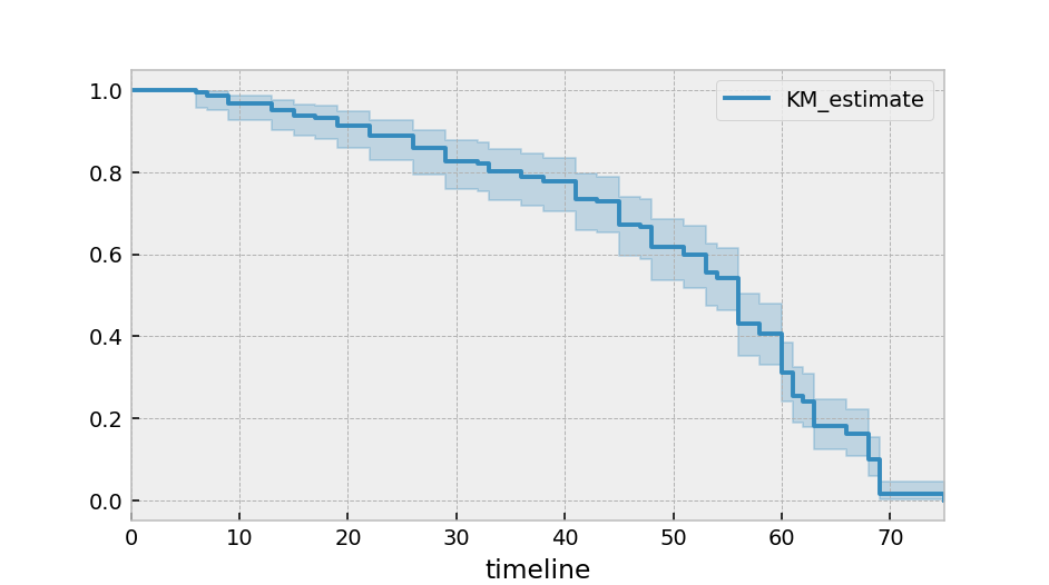
After calling the fit() method, we have access to new properties like survival_function_ and methods like plot(). The latter is a wrapper around Panda’s internal plotting library.
kmf.survival_function_
kmf.cumulative_density_
kmf.plot_survival_function()
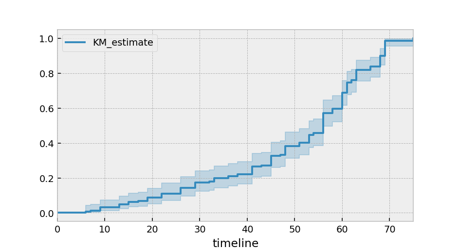
Alternatively, you can plot the cumulative density function:
kmf.plot_cumulative_density()
By specifying the timeline keyword argument in fit(), we can change how the above models are indexed:
kmf.fit(T, E, timeline=range(0, 100, 2))

kmf.survival_function_   # index is now the same as range(0, 100, 2)
kmf.confidence_interval_ # index is now the same as range(0, 100, 2)
A useful summary stat is the median survival time, which represents when 50% of the population has died:
from lifelines.utils import median_survival_times

median_ = kmf.median_survival_time_
median_confidence_interval_ = median_survival_times(kmf.confidence_interval_)
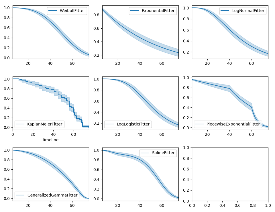
Instead of the Kaplan-Meier estimator, you may be interested in a parametric model. lifelines has builtin parametric models. For example, Weibull, Log-Normal, Log-Logistic, and more.
import matplotlib.pyplot as plt
import numpy as np
from lifelines import *

fig, axes = plt.subplots(3, 3, figsize=(13.5, 7.5))

kmf = KaplanMeierFitter().fit(T, E, label='KaplanMeierFitter')
wbf = WeibullFitter().fit(T, E, label='WeibullFitter')
exf = ExponentialFitter().fit(T, E, label='ExponentialFitter')
lnf = LogNormalFitter().fit(T, E, label='LogNormalFitter')
llf = LogLogisticFitter().fit(T, E, label='LogLogisticFitter')
pwf = PiecewiseExponentialFitter([40, 60]).fit(T, E, label='PiecewiseExponentialFitter')
ggf = GeneralizedGammaFitter().fit(T, E, label='GeneralizedGammaFitter')
sf = SplineFitter(np.percentile(T.loc[E.astype(bool)], [0, 50, 100])).fit(T, E, label='SplineFitter')

wbf.plot_survival_function(ax=axes[0][0])
exf.plot_survival_function(ax=axes[0][1])
lnf.plot_survival_function(ax=axes[0][2])
kmf.plot_survival_function(ax=axes[1][0])
llf.plot_survival_function(ax=axes[1][1])
pwf.plot_survival_function(ax=axes[1][2])
ggf.plot_survival_function(ax=axes[2][0])
sf.plot_survival_function(ax=axes[2][1])
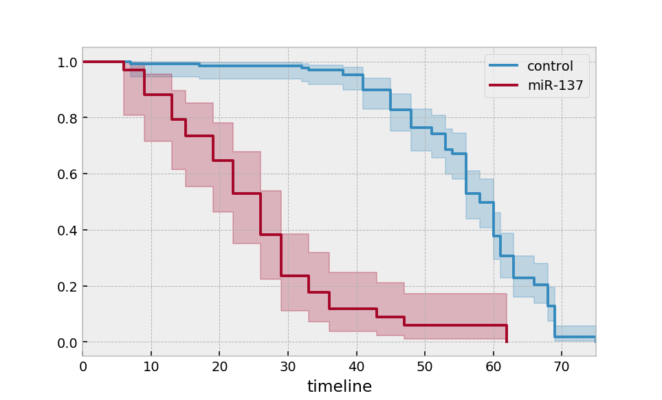
Multiple groups
groups = df['group']
ix = (groups == 'miR-137')

kmf.fit(T[~ix], E[~ix], label='control')
ax = kmf.plot_survival_function()

kmf.fit(T[ix], E[ix], label='miR-137')
ax = kmf.plot_survival_function(ax=ax)
Alternatively, for many more groups and more “pandas-esque”:
ax = plt.subplot(111)

kmf = KaplanMeierFitter()

for name, grouped_df in df.groupby('group'):
    kmf.fit(grouped_df["T"], grouped_df["E"], label=name)
    kmf.plot_survival_function(ax=ax)
Similar functionality exists for the NelsonAalenFitter:
from lifelines import NelsonAalenFitter
naf = NelsonAalenFitter()
naf.fit(T, event_observed=E)
but instead of a survival_function_ being exposed, a cumulative_hazard_ is.
Note
Similar to Scikit-Learn, all statistically estimated quantities append an underscore to the property name.
Note
More detailed docs about estimating the survival function and cumulative hazard are available in Survival analysis with lifelines.
Getting data in the right format
Often you’ll have data that looks like::
*start_time1*, *end_time1*
*start_time2*, *end_time2*
*start_time3*, None
*start_time4*, *end_time4*
lifelines has some utility functions to transform this dataset into duration and censoring vectors. The most common one is lifelines.utils.datetimes_to_durations().
from lifelines.utils import datetimes_to_durations

# start_times is a vector or list of datetime objects or datetime strings
# end_times is a vector or list of (possibly missing) datetime objects or datetime strings
T, E = datetimes_to_durations(start_times, end_times, freq='h')
Perhaps you are interested in viewing the survival table given some durations and censoring vectors. The function lifelines.utils.survival_table_from_events() will help with that:
from lifelines.utils import survival_table_from_events

table = survival_table_from_events(T, E)
print(table.head())

"""
          removed  observed  censored  entrance  at_risk
event_at
0               0         0         0       163      163
6               1         1         0         0      163
7               2         1         1         0      162
9               3         3         0         0      160
13              3         3         0         0      157
"""
Survival regression
While the above KaplanMeierFitter model is useful, it only gives us an “average” view of the population. Often we have specific data at the individual level that we would like to use. For this, we turn to survival regression.
Note
More detailed documentation and tutorials are available in Survival Regression.
The dataset for regression models is different than the datasets above. All the data, including durations, censored indicators and covariates must be contained in a Pandas DataFrame.
from lifelines.datasets import load_regression_dataset
regression_dataset = load_regression_dataset() # a Pandas DataFrame
A regression model is instantiated, and a model is fit to a dataset using fit. The duration column and event column are specified in the call to fit. Below we model our regression dataset using the Cox proportional hazard model, full docs here.
from lifelines import CoxPHFitter

# Using Cox Proportional Hazards model
cph = CoxPHFitter()
cph.fit(regression_dataset, 'T', event_col='E')
cph.print_summary()

"""
<lifelines.CoxPHFitter: fitted with 200 total observations, 11 right-censored observations>
             duration col = 'T'
                event col = 'E'
      baseline estimation = breslow
   number of observations = 200
number of events observed = 189
   partial log-likelihood = -807.62
         time fit was run = 2020-06-21 12:26:28 UTC

---
       coef  exp(coef)   se(coef)   coef lower 95%   coef upper 95%  exp(coef) lower 95%  exp(coef) upper 95%
var1   0.22       1.25       0.07             0.08             0.37                 1.08                 1.44
var2   0.05       1.05       0.08            -0.11             0.21                 0.89                 1.24
var3   0.22       1.24       0.08             0.07             0.37                 1.07                 1.44

        z      p   -log2(p)
var1 2.99 <0.005       8.49
var2 0.61   0.54       0.89
var3 2.88 <0.005       7.97
---
Concordance = 0.58
Partial AIC = 1621.24
log-likelihood ratio test = 15.54 on 3 df
-log2(p) of ll-ratio test = 9.47
"""

cph.plot()
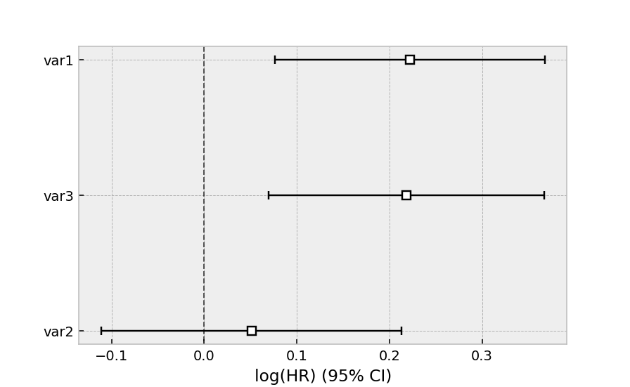
The same dataset, but with a Weibull accelerated failure time model. This model was two parameters (see docs here), and we can choose to model both using our covariates or just one. Below we model just the scale parameter, lambda_.
from lifelines import WeibullAFTFitter

wft = WeibullAFTFitter()
wft.fit(regression_dataset, 'T', event_col='E')
wft.print_summary()

"""
<lifelines.WeibullAFTFitter: fitted with 200 total observations, 11 right-censored observations>
             duration col = 'T'
                event col = 'E'
   number of observations = 200
number of events observed = 189
           log-likelihood = -504.48
         time fit was run = 2020-06-21 12:27:05 UTC

---
                     coef  exp(coef)   se(coef)   coef lower 95%   coef upper 95%  exp(coef) lower 95%  exp(coef) upper 95%
lambda_ var1        -0.08       0.92       0.02            -0.13            -0.04                 0.88                 0.97
        var2        -0.02       0.98       0.03            -0.07             0.04                 0.93                 1.04
        var3        -0.08       0.92       0.02            -0.13            -0.03                 0.88                 0.97
        Intercept   2.53      12.57       0.05             2.43             2.63                11.41                13.85
rho_    Intercept   1.09       2.98       0.05             0.99             1.20                 2.68                 3.32

                       z      p   -log2(p)
lambda_ var1       -3.45 <0.005      10.78
        var2       -0.56   0.57       0.80
        var3       -3.33 <0.005      10.15
        Intercept 51.12 <0.005        inf
rho_    Intercept 20.12 <0.005     296.66
---
Concordance = 0.58
AIC = 1018.97
log-likelihood ratio test = 19.73 on 3 df
-log2(p) of ll-ratio test = 12.34
"""

wft.plot()
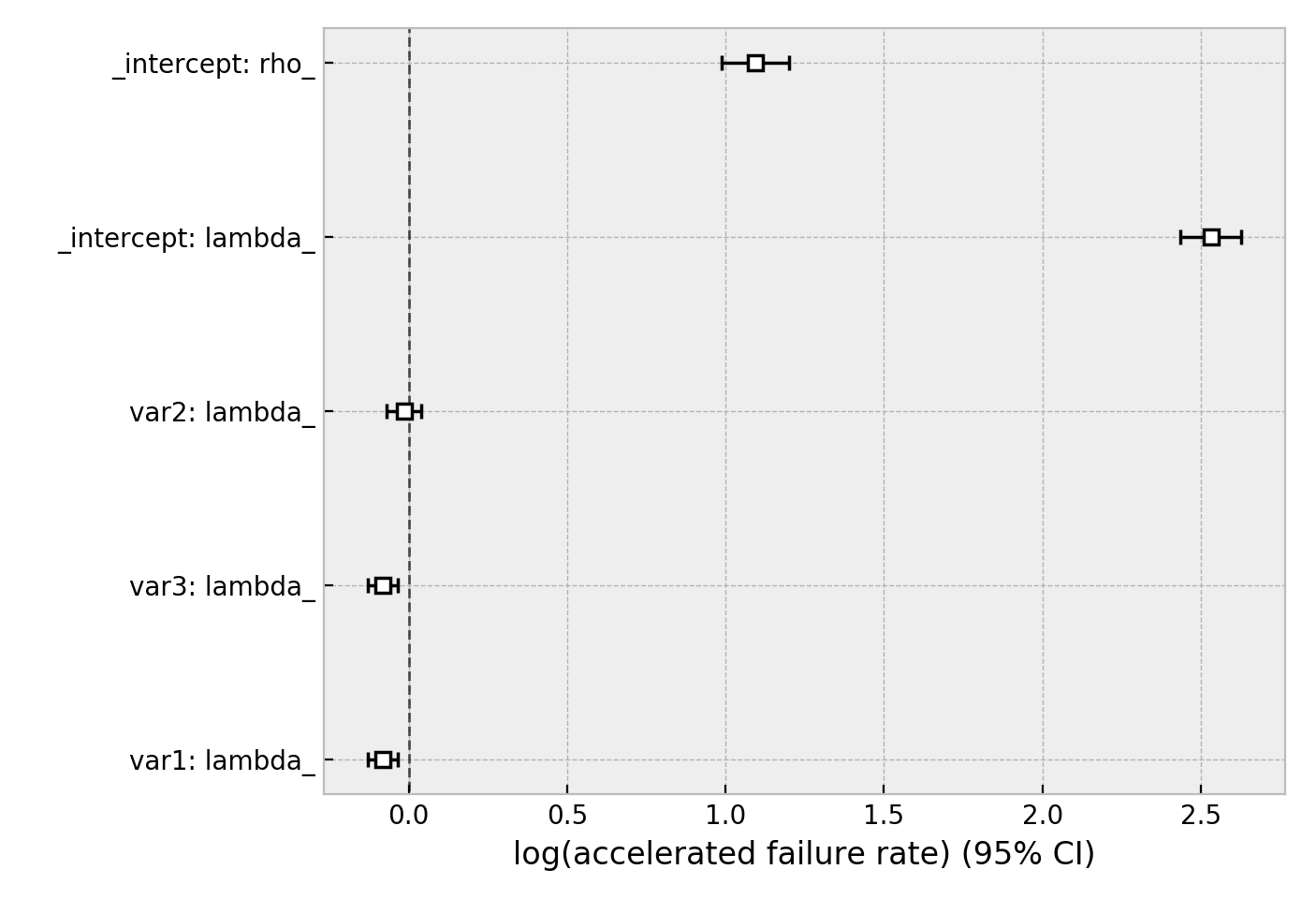
Other AFT models are available as well, see here. An alternative regression model is Aalen’s Additive model, which has time-varying hazards:
# Using Aalen's Additive model
from lifelines import AalenAdditiveFitter
aaf = AalenAdditiveFitter(fit_intercept=False)
aaf.fit(regression_dataset, 'T', event_col='E')
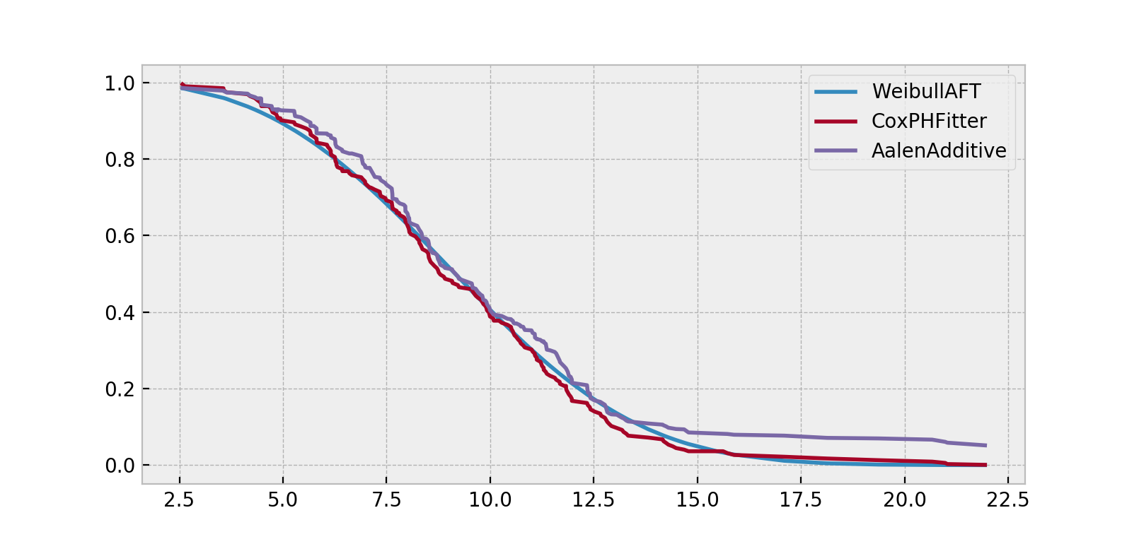
Along with CoxPHFitter and WeibullAFTFitter, after fitting you’ll have access to properties like summary and methods like plot, predict_cumulative_hazards, and predict_survival_function. The latter two methods require an additional argument of covariates:
X = regression_dataset.loc[0]

ax = wft.predict_survival_function(X).rename(columns={0:'WeibullAFT'}).plot()
cph.predict_survival_function(X).rename(columns={0:'CoxPHFitter'}).plot(ax=ax)
aaf.predict_survival_function(X).rename(columns={0:'AalenAdditive'}).plot(ax=ax)
Note
More detailed documentation and tutorials are available in Survival Regression.