
Time-lagged conversion rates and cure models
Suppose in our population we have a subpopulation that will never experience the event of interest. Or, for some subjects the event will occur so far in the future that it’s essentially at time infinity. The survival function should not asymptotically approach zero, but some positive value. Models that describe this are sometimes called cure models (i.e. the subject is “cured” of death and hence no longer susceptible) or time-lagged conversion models.
There’s a serious fault in using parametric models for these types of problems that non-parametric models don’t have. The most common parametric models like Weibull, Log-Normal, etc. all have strictly increasing cumulative hazard functions, which means the corresponding survival function will always converge to 0.
Let’s look at an example of this problem. Below I generated some data that has individuals who will not experience the event, not matter how long we wait.
[1]:
%matplotlib inline
%config InlineBackend.figure_format = 'retina'

from matplotlib import pyplot as plt
import autograd.numpy as np
from autograd.scipy.special import expit, logit
import pandas as pd
plt.style.use('bmh')
[2]:
N = 200
U = np.random.rand(N)
T = -(logit(-np.log(U) / 0.5) - np.random.exponential(2, N) - 6.00) / 0.50

E = ~np.isnan(T)
T[np.isnan(T)] = 50
[5]:
from lifelines import KaplanMeierFitter
kmf = KaplanMeierFitter().fit(T, E)
kmf.plot(figsize=(8,4))
plt.ylim(0, 1);
plt.title("Survival function estimated by KaplanMeier")
[5]:
Text(0.5, 1.0, 'Survival function estimated by KaplanMeier')
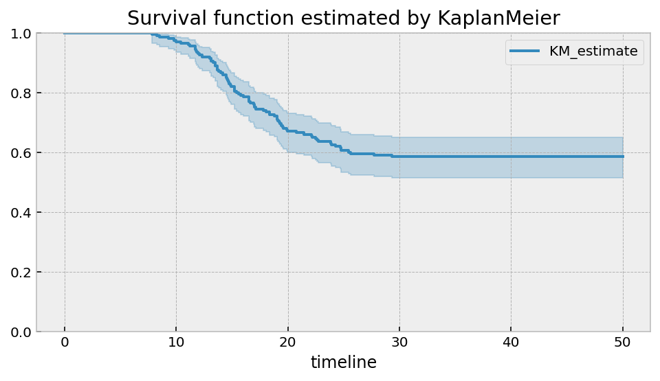
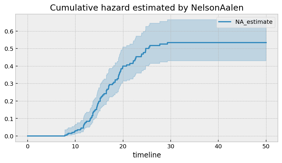
It should be clear that there is an asymptote at around 0.6. The non-parametric model will always show this. If this is true, then the cumulative hazard function should have a horizontal asymptote as well. Let’s use the Nelson-Aalen model to see this.
[6]:
from lifelines import NelsonAalenFitter

naf = NelsonAalenFitter().fit(T, E)
naf.plot(figsize=(8,4))
plt.title("Cumulative hazard estimated by NelsonAalen")
[6]:
Text(0.5, 1.0, 'Cumulative hazard estimated by NelsonAalen')
However, when we try a parametric model, we will see that it won’t extrapolate very well. Let’s use the flexible two parameter LogLogisticFitter model.
[11]:
from lifelines import LogLogisticFitter

fig, ax = plt.subplots(nrows=1, ncols=2, figsize=(12, 4))

t = np.linspace(0, 40)
llf = LogLogisticFitter().fit(T, E, timeline=t)

t = np.linspace(0, 100)
llf = LogLogisticFitter().fit(T, E, timeline=t)

llf.plot_survival_function(ax=ax[0])
kmf.plot(ax=ax[0])

llf.plot_cumulative_hazard(ax=ax[1])
naf.plot(ax=ax[1])
[11]:
<AxesSubplot:xlabel='timeline'>
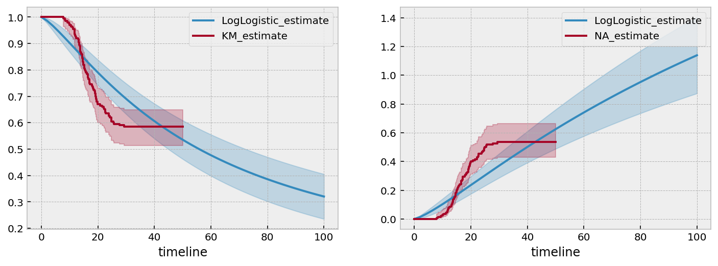
The LogLogistic model does a quite terrible job of capturing the not only the asymptotes, but also the intermediate values as well. If we extended the survival function out further, we would see that it eventually nears 0.
Custom parametric models to handle asymptotes
Focusing on modeling the cumulative hazard function, what we would like is a function that increases up to a limit and then tapers off to an asymptote. We can think long and hard about these (I did), but there’s a family of functions that have this property that we are very familiar with: cumulative distribution functions! By their nature, they will asympotically approach 1. And, they are readily available in the SciPy and autograd libraries. So our new model of the cumulative hazard function is:
where \(c\) is the (unknown) horizontal asymptote, and \(\theta\) is a vector of (unknown) parameters for the CDF, \(F\).
We can create a custom cumulative hazard model using ParametricUnivariateFitter (for a tutorial on how to create custom models, see this here). Let’s choose the Normal CDF for our model.
Remember we must use the imports from autograd for this, i.e. from autograd.scipy.stats import norm.
[13]:
from autograd.scipy.stats import norm
from lifelines.fitters import ParametricUnivariateFitter


class UpperAsymptoteFitter(ParametricUnivariateFitter):

    _fitted_parameter_names = ["c_", "mu_", "sigma_"]

    _bounds = ((0, None), (None, None), (0, None))

    def _cumulative_hazard(self, params, times):
        c, mu, sigma = params
        return c * norm.cdf((times - mu) / sigma, loc=0, scale=1)
[14]:
uaf = UpperAsymptoteFitter().fit(T, E)
uaf.print_summary(3)
uaf.plot(figsize=(8,4))
| model | lifelines.UpperAsymptoteFitter |
|---|---|
| number of observations | 200 |
| number of events observed | 83 |
| log-likelihood | -382.304 |
| hypothesis | c_ != 1, mu_ != 0, sigma_ != 1 |
| coef | se(coef) | coef lower 95% | coef upper 95% | z | p | -log2(p) | |
|---|---|---|---|---|---|---|---|
| c_ | 0.539 | 0.060 | 0.422 | 0.657 | -7.701 | <0.0005 | 46.069 |
| mu_ | 17.397 | 0.527 | 16.364 | 18.429 | 33.015 | <0.0005 | 791.632 |
| sigma_ | 4.746 | 0.369 | 4.022 | 5.470 | 10.142 | <0.0005 | 77.880 |
| AIC | 770.608 |
|---|
[14]:
<AxesSubplot:>
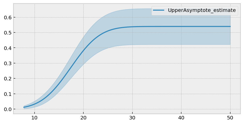
We get a lovely asympotical cumulative hazard. The summary table suggests that the best value of \(c\) is 0.586. This can be translated into the survival function asymptote by \(\exp(-0.586) \approx 0.56\).
Let’s compare this fit to the non-parametric models.
[15]:
fig, ax = plt.subplots(nrows=2, ncols=2, figsize=(10, 6))

t = np.linspace(0, 40)
uaf = UpperAsymptoteFitter().fit(T, E, timeline=t)

uaf.plot_survival_function(ax=ax[0][0])
kmf.plot(ax=ax[0][0])

uaf.plot_cumulative_hazard(ax=ax[0][1])
naf.plot(ax=ax[0][1])

t = np.linspace(0, 100)
uaf = UpperAsymptoteFitter().fit(T, E, timeline=t)
uaf.plot_survival_function(ax=ax[1][0])
kmf.survival_function_.plot(ax=ax[1][0])

uaf.plot_cumulative_hazard(ax=ax[1][1])
naf.plot(ax=ax[1][1])
[15]:
<AxesSubplot:xlabel='timeline'>
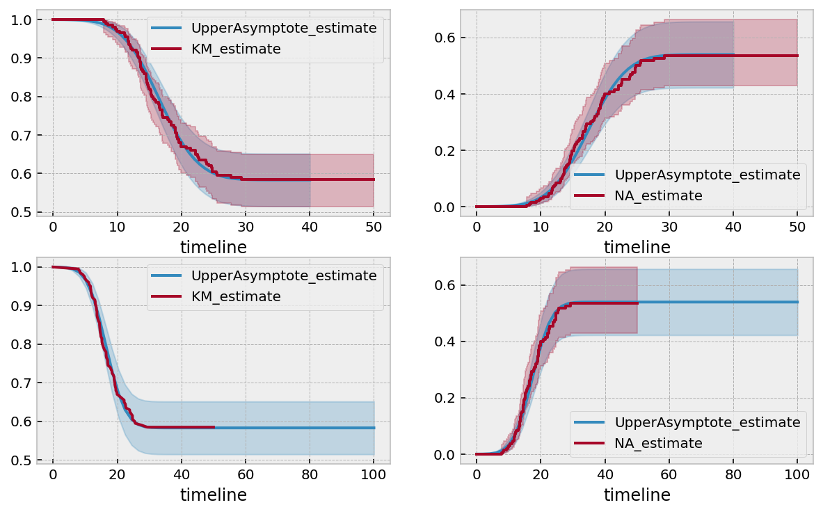
I wasn’t expecting this good of a fit. But there it is. This was some artificial data, but let’s try this technique on some real life data.
[18]:
from lifelines.datasets import load_leukemia, load_kidney_transplant

T, E = load_leukemia()['t'], load_leukemia()['status']
uaf.fit(T, E)
ax = uaf.plot_survival_function(figsize=(8,4))
uaf.print_summary()

kmf.fit(T, E).plot(ax=ax, ci_show=False)
print("---")
print("Estimated lower bound: {:.2f} ({:.2f}, {:.2f})".format(
        np.exp(-uaf.summary.loc['c_', 'coef']),
        np.exp(-uaf.summary.loc['c_', 'coef upper 95%']),
        np.exp(-uaf.summary.loc['c_', 'coef upper 95%']),
    )
)
| model | lifelines.UpperAsymptoteFitter |
|---|---|
| number of observations | 42 |
| number of events observed | 30 |
| log-likelihood | -118.60 |
| hypothesis | c_ != 1, mu_ != 0, sigma_ != 1 |
| coef | se(coef) | coef lower 95% | coef upper 95% | z | p | -log2(p) | |
|---|---|---|---|---|---|---|---|
| c_ | 1.63 | 0.36 | 0.94 | 2.33 | 1.78 | 0.07 | 3.75 |
| mu_ | 13.44 | 1.73 | 10.06 | 16.82 | 7.79 | <0.005 | 47.07 |
| sigma_ | 7.03 | 1.07 | 4.94 | 9.12 | 5.65 | <0.005 | 25.91 |
| AIC | 243.20 |
|---|
---
Estimated lower bound: 0.20 (0.10, 0.10)
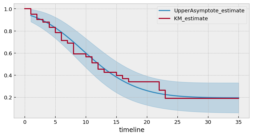
So we might expect that about 20% will not have the even in this population (but make note of the large CI bounds too!)
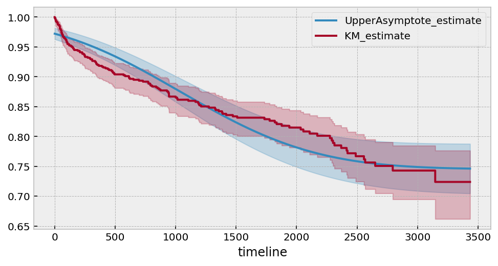
[21]:
# Another, less obvious, dataset.

T, E = load_kidney_transplant()['time'], load_kidney_transplant()['death']
uaf.fit(T, E)
ax = uaf.plot_survival_function(figsize=(8,4))
uaf.print_summary()

kmf.fit(T, E).plot(ax=ax)
print("---")
print("Estimated lower bound: {:.2f} ({:.2f}, {:.2f})".format(
        np.exp(-uaf.summary.loc['c_', 'coef']),
        np.exp(-uaf.summary.loc['c_', 'coef upper 95%']),
        np.exp(-uaf.summary.loc['c_', 'coef lower 95%']),
    )
)
| model | lifelines.UpperAsymptoteFitter |
|---|---|
| number of observations | 863 |
| number of events observed | 140 |
| log-likelihood | -1458.88 |
| hypothesis | c_ != 1, mu_ != 0, sigma_ != 1 |
| coef | se(coef) | coef lower 95% | coef upper 95% | z | p | -log2(p) | |
|---|---|---|---|---|---|---|---|
| c_ | 0.29 | 0.03 | 0.24 | 0.35 | -24.37 | <0.005 | 433.49 |
| mu_ | 1139.88 | 101.60 | 940.75 | 1339.01 | 11.22 | <0.005 | 94.62 |
| sigma_ | 872.59 | 66.31 | 742.62 | 1002.56 | 13.14 | <0.005 | 128.67 |
| AIC | 2923.76 |
|---|
---
Estimated lower bound: 0.75 (0.70, 0.79)
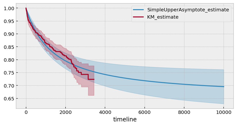
Using alternative functional forms
An even simpler model might look like \(c \left(1 - \frac{1}{\lambda t + 1}\right)\), however this model cannot handle any “inflection points” like our artificial dataset has above. However, it works well for this Lung dataset.
With all parametric models, one important feature is the ability to extrapolate to unforeseen times.
[22]:
from autograd.scipy.stats import norm
from lifelines.fitters import ParametricUnivariateFitter

class SimpleUpperAsymptoteFitter(ParametricUnivariateFitter):

    _fitted_parameter_names = ["c_", "lambda_"]

    _bounds = ((0, None), (0, None))

    def _cumulative_hazard(self, params, times):
        c, lambda_ = params
        return c * (1 -  1 /(lambda_ * times + 1))
[23]:
# Another, less obvious, dataset.

saf = SimpleUpperAsymptoteFitter().fit(T, E, timeline=np.arange(1, 10000))
ax = saf.plot_survival_function(figsize=(8,4))
saf.print_summary(4)

kmf.fit(T, E).plot(ax=ax)
print("---")
print("Estimated lower bound: {:.2f} ({:.2f}, {:.2f})".format(
        np.exp(-saf.summary.loc['c_', 'coef']),
        np.exp(-saf.summary.loc['c_', 'coef upper 95%']),
        np.exp(-saf.summary.loc['c_', 'coef lower 95%']),
    )
)
| model | lifelines.SimpleUpperAsymptoteFitter |
|---|---|
| number of observations | 863 |
| number of events observed | 140 |
| log-likelihood | -1392.1610 |
| hypothesis | c_ != 1, lambda_ != 1 |
| coef | se(coef) | coef lower 95% | coef upper 95% | z | p | -log2(p) | |
|---|---|---|---|---|---|---|---|
| c_ | 0.4252 | 0.0717 | 0.2847 | 0.5658 | -8.0151 | <5e-05 | 49.6912 |
| lambda_ | 0.0006 | 0.0002 | 0.0003 | 0.0009 | -5982.3551 | <5e-05 | inf |
| AIC | 2788.3221 |
|---|
---
Estimated lower bound: 0.65 (0.57, 0.75)
Probabilistic cure models
The models above are good at fitting to the data, but they offer less common interpretation of survival models. It would be nice to be able to use common survival models and have some “cure” component. Let’s suppose that for individuals that will experience the event of interest, their survival distribution is a Weibull, denoted \(S_W(t)\). For a random selected individual in the population, their survival curve, \(S(t)\), is:
Even though it’s in an unconventional form, we can still determine the cumulative hazard (which is the negative logarithm of the survival function):
[24]:
from autograd import numpy as np
from lifelines.fitters import ParametricUnivariateFitter

class CureFitter(ParametricUnivariateFitter):

    _fitted_parameter_names = ["p_", "lambda_", "rho_"]

    _bounds = ((0, 1), (0, None), (0, None))

    def _cumulative_hazard(self, params, T):
        p, lambda_, rho_ = params
        sf = np.exp(-(T / lambda_) ** rho_)
        return -np.log(p + (1-p) * sf)
[25]:
cure_model = CureFitter().fit(T, E, timeline=np.arange(1, 10000))
ax = cure_model.plot_survival_function(figsize=(8,4))
cure_model.print_summary(4)

kmf.fit(T, E).plot(ax=ax)
print("---")
print("Estimated lower bound: {:.2f} ({:.2f}, {:.2f})".format(
        cure_model.summary.loc['p_', 'coef'],
        cure_model.summary.loc['p_', 'coef upper 95%'],
        cure_model.summary.loc['p_', 'coef lower 95%'],
    )
)
| model | lifelines.CureFitter |
|---|---|
| number of observations | 863 |
| number of events observed | 140 |
| log-likelihood | -1385.1617 |
| hypothesis | p_ != 0.5, lambda_ != 1, rho_ != 1 |
| coef | se(coef) | coef lower 95% | coef upper 95% | z | p | -log2(p) | |
|---|---|---|---|---|---|---|---|
| p_ | 0.1006 | 1.3053 | -2.4577 | 2.6590 | -0.3059 | 0.7596 | 0.3966 |
| lambda_ | 17393.6107 | 48891.6027 | -78432.1698 | 113219.3911 | 0.3557 | 0.7220 | 0.4699 |
| rho_ | 0.6382 | 0.0791 | 0.4831 | 0.7932 | -4.5739 | <5e-05 | 17.6725 |
| AIC | 2776.3234 |
|---|
---
Estimated lower bound: 0.10 (2.66, -2.46)
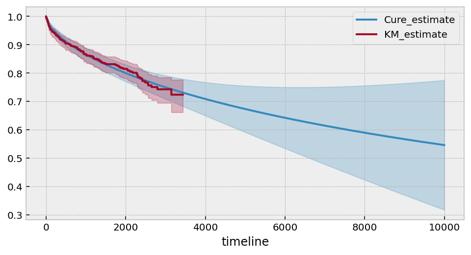
Under this model, it suggests that only ~10% of subjects are ever cured (however, there is a lot of variance in the estimate of the \(p\) parameter).