---

%matplotlib inline
%config InlineBackend.figure_format = 'retina'

from matplotlib import pyplot as plt
from lifelines import CoxPHFitter
import numpy as np
import pandas as pd

Testing the proportional hazard assumptions

This Jupyter notebook is a small tutorial on how to test and fix proportional hazard problems. An important question to first ask is: do I need to care about the proportional hazard assumption? - often the answer is no.

The proportional hazard assumption is that all individuals have the same hazard function, but a unique scaling factor infront. So the shape of the hazard function is the same for all individuals, and only a scalar multiple changes per individual.

\[h_i(t) = a_i h(t)\]

At the core of the assumption is that \(a_i\) is not time varying, that is, \(a_i(t) = a_i\). Further more, if we take the ratio of this with another subject (called the hazard ratio):

\[\frac{h_i(t)}{h_j(t)} = \frac{a_i h(t)}{a_j h(t)} = \frac{a_i}{a_j}\]

is constant for all \(t\). In this tutorial we will test this non-time varying assumption, and look at ways to handle violations.

from lifelines.datasets import load_rossi
rossi = load_rossi()
cph = CoxPHFitter()

cph.fit(rossi, 'week', 'arrest')

<lifelines.CoxPHFitter: fitted with 432 total observations, 318 right-censored observations>

cph.print_summary(model="untransformed variables", decimals=3)

model	lifelines.CoxPHFitter
duration col	'week'
event col	'arrest'
baseline estimation	breslow
number of observations	432
number of events observed	114
partial log-likelihood	-658.748
time fit was run	2020-07-26 22:15:39 UTC
model	untransformed variables

	coef	exp(coef)	se(coef)	coef lower 95%	coef upper 95%	exp(coef) lower 95%	exp(coef) upper 95%	z	p	-log2(p)
covariate
fin	-0.379	0.684	0.191	-0.755	-0.004	0.470	0.996	-1.983	0.047	4.398
age	-0.057	0.944	0.022	-0.101	-0.014	0.904	0.986	-2.611	0.009	6.791
race	0.314	1.369	0.308	-0.290	0.918	0.748	2.503	1.019	0.308	1.698
wexp	-0.150	0.861	0.212	-0.566	0.266	0.568	1.305	-0.706	0.480	1.058
mar	-0.434	0.648	0.382	-1.182	0.315	0.307	1.370	-1.136	0.256	1.965
paro	-0.085	0.919	0.196	-0.469	0.299	0.626	1.348	-0.434	0.665	0.589
prio	0.091	1.096	0.029	0.035	0.148	1.036	1.159	3.194	0.001	9.476

Concordance	0.640
Partial AIC	1331.495
log-likelihood ratio test	33.266 on 7 df
-log2(p) of ll-ratio test	15.370

Checking assumptions with check_assumptions

New to lifelines 0.16.0 is the CoxPHFitter.check_assumptions method. This method will compute statistics that check the proportional hazard assumption, produce plots to check assumptions, and more. Also included is an option to display advice to the console. Here’s a breakdown of each information displayed:

• Presented first are the results of a statistical test to test for any time-varying coefficients. A time-varying coefficient imply a covariate’s influence relative to the baseline changes over time. This implies a violation of the proportional hazard assumption. For each variable, we transform time four times (these are common transformations of time to perform). If lifelines rejects the null (that is, lifelines rejects that the coefficient is not time-varying), we report this to the user.

• Some advice is presented on how to correct the proportional hazard violation based on some summary statistics of the variable.

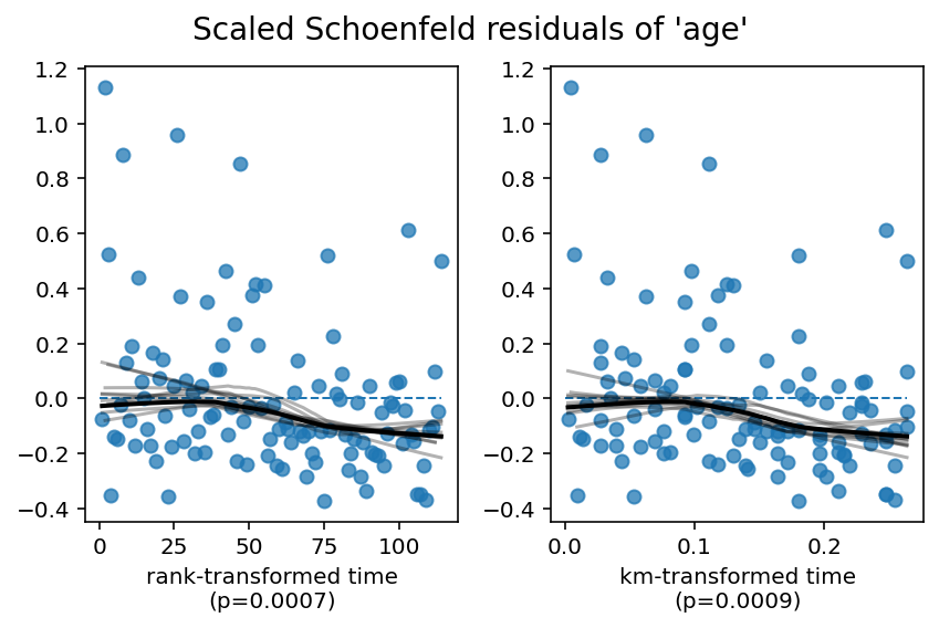
• As a compliment to the above statistical test, if the option show_plots = True is specified, visual plots of the the scaled Schoenfeld residuals are presented for all covariates against the four time transformations. A fitted lowess is also presented, along with 10 bootstrapped lowess lines (as an approximation to the confidence interval of the original lowess line). Ideally, this lowess line is constant (flat). Deviations away from the constant line are violations of the PH assumption.

Why the scaled Schoenfeld residuals?

This section can be skipped on first read. Let \(s_{t,j}\) denote the scaled Schoenfeld residuals of variable \(j\) at time \(t\), \(\hat{\beta_j}\) denote the maximum-likelihood estimate of the \(j\)th variable, and \(\beta_j(t)\) a time-varying coefficient in (fictional) alternative model that allows for time-varying coefficients. Therneau and Grambsch showed that.

\[E[s_{t,j}] + \hat{\beta_j} = \beta_j(t)\]

The proportional hazard assumption implies that \(\hat{\beta_j} = \beta_j(t)\), hence \(E[s_{t,j}] = 0\). This is what the above proportional hazard test is testing. Visually, plotting \(s_{t,j}\) over time (or some transform of time), is a good way to see violations of \(E[s_{t,j}] = 0\), along with the statisical test.

cph.check_assumptions(rossi, p_value_threshold=0.05, show_plots=True)

The ``p_value_threshold`` is set at 0.05. Even under the null hypothesis of no violations, some
covariates will be below the threshold by chance. This is compounded when there are many covariates.
Similarly, when there are lots of observations, even minor deviances from the proportional hazard
assumption will be flagged.

With that in mind, it's best to use a combination of statistical tests and visual tests to determine
the most serious violations. Produce visual plots using ``check_assumptions(..., show_plots=True)``
and looking for non-constant lines. See link [A] below for a full example.

null_distribution	chi squared
degrees_of_freedom	1
model	<lifelines.CoxPHFitter: fitted with 432 total ...
test_name	proportional_hazard_test

		test_statistic	p
age	km	11.03	<0.005
	rank	11.45	<0.005
fin	km	0.02	0.89
	rank	0.02	0.90
mar	km	0.60	0.44
	rank	0.71	0.40
paro	km	0.12	0.73
	rank	0.13	0.71
prio	km	0.02	0.88
	rank	0.02	0.89
race	km	1.44	0.23
	rank	1.43	0.23
wexp	km	7.48	0.01
	rank	7.31	0.01

1. Variable 'age' failed the non-proportional test: p-value is 0.0007.

   Advice 1: the functional form of the variable 'age' might be incorrect. That is, there may be
non-linear terms missing. The proportional hazard test used is very sensitive to incorrect
functional forms. See documentation in link [D] below on how to specify a functional form.

   Advice 2: try binning the variable 'age' using pd.cut, and then specify it in `strata=['age',
...]` in the call in `.fit`. See documentation in link [B] below.

   Advice 3: try adding an interaction term with your time variable. See documentation in link [C]
below.


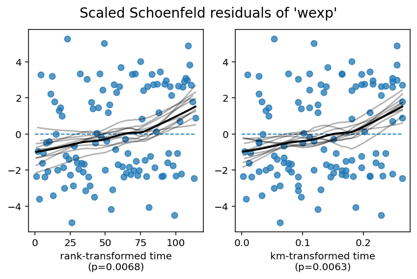
2. Variable 'wexp' failed the non-proportional test: p-value is 0.0063.

   Advice: with so few unique values (only 2), you can include `strata=['wexp', ...]` in the call in
`.fit`. See documentation in link [E] below.

---
[A]  https://lifelines.readthedocs.io/en/latest/jupyter_notebooks/Proportional%20hazard%20assumption.html
[B]  https://lifelines.readthedocs.io/en/latest/jupyter_notebooks/Proportional%20hazard%20assumption.html#Bin-variable-and-stratify-on-it
[C]  https://lifelines.readthedocs.io/en/latest/jupyter_notebooks/Proportional%20hazard%20assumption.html#Introduce-time-varying-covariates
[D]  https://lifelines.readthedocs.io/en/latest/jupyter_notebooks/Proportional%20hazard%20assumption.html#Modify-the-functional-form
[E]  https://lifelines.readthedocs.io/en/latest/jupyter_notebooks/Proportional%20hazard%20assumption.html#Stratification

Alternatively, you can use the proportional hazard test outside of check_assumptions:

from lifelines.statistics import proportional_hazard_test

results = proportional_hazard_test(cph, rossi, time_transform='rank')
results.print_summary(decimals=3, model="untransformed variables")

time_transform	rank
null_distribution	chi squared
degrees_of_freedom	1
model	untransformed variables
test_name	proportional_hazard_test

	test_statistic	p
age	11.453	0.001
fin	0.015	0.902
mar	0.709	0.400
paro	0.134	0.714
prio	0.019	0.891
race	1.426	0.232
wexp	7.315	0.007

Stratification

In the advice above, we can see that wexp has small cardinality, so we can easily fix that by specifying it in the strata. What does the strata do? Let’s go back to the proportional hazard assumption.

In the introduction, we said that the proportional hazard assumption was that

\[h_i(t) = a_i h(t)\]

In a simple case, it may be that there are two subgroups that have very different baseline hazards. That is, we can split the dataset into subsamples based on some variable (we call this the stratifying variable), run the Cox model on all subsamples, and compare their baseline hazards. If these baseline hazards are very different, then clearly the formula above is wrong - the \(h(t)\) is some weighted average of the subgroups’ baseline hazards. This ill fitting average baseline can cause \(a_i\) to have time-dependent influence. A better model might be:

\[h_{i |i\in G}(t) = a_i h_G(t)\]

where now we have a unique baseline hazard per subgroup \(G\). Because of the way the Cox model is designed, inference of the coefficients is identical (expect now there are more baseline hazards, and no variation of the stratifying variable within a subgroup \(G\)).

cph.fit(rossi, 'week', 'arrest', strata=['wexp'])
cph.print_summary(model="wexp in strata")

model	lifelines.CoxPHFitter
duration col	'week'
event col	'arrest'
strata	[wexp]
baseline estimation	breslow
number of observations	432
number of events observed	114
partial log-likelihood	-580.89
time fit was run	2020-07-26 22:15:41 UTC
model	wexp in strata

	coef	exp(coef)	se(coef)	coef lower 95%	coef upper 95%	exp(coef) lower 95%	exp(coef) upper 95%	z	p	-log2(p)
covariate
fin	-0.38	0.68	0.19	-0.76	-0.01	0.47	0.99	-1.99	0.05	4.42
age	-0.06	0.94	0.02	-0.10	-0.01	0.90	0.99	-2.64	0.01	6.91
race	0.31	1.36	0.31	-0.30	0.91	0.74	2.49	1.00	0.32	1.65
mar	-0.45	0.64	0.38	-1.20	0.29	0.30	1.34	-1.19	0.23	2.09
paro	-0.08	0.92	0.20	-0.47	0.30	0.63	1.35	-0.42	0.67	0.57
prio	0.09	1.09	0.03	0.03	0.15	1.04	1.16	3.16	<0.005	9.33

Concordance	0.61
Partial AIC	1173.77
log-likelihood ratio test	23.77 on 6 df
-log2(p) of ll-ratio test	10.77

cph.check_assumptions(rossi, show_plots=True)

The ``p_value_threshold`` is set at 0.01. Even under the null hypothesis of no violations, some
covariates will be below the threshold by chance. This is compounded when there are many covariates.
Similarly, when there are lots of observations, even minor deviances from the proportional hazard
assumption will be flagged.

With that in mind, it's best to use a combination of statistical tests and visual tests to determine
the most serious violations. Produce visual plots using ``check_assumptions(..., show_plots=True)``
and looking for non-constant lines. See link [A] below for a full example.

null_distribution	chi squared
degrees_of_freedom	1
model	<lifelines.CoxPHFitter: fitted with 432 total ...
test_name	proportional_hazard_test

		test_statistic	p
age	km	11.29	<0.005
	rank	4.62	0.03
fin	km	0.02	0.90
	rank	0.05	0.83
mar	km	0.53	0.47
	rank	1.31	0.25
paro	km	0.09	0.76
	rank	0.00	0.97
prio	km	0.02	0.89
	rank	0.02	0.90
race	km	1.47	0.23
	rank	0.64	0.42

1. Variable 'age' failed the non-proportional test: p-value is 0.0008.

   Advice 1: the functional form of the variable 'age' might be incorrect. That is, there may be
non-linear terms missing. The proportional hazard test used is very sensitive to incorrect
functional forms. See documentation in link [D] below on how to specify a functional form.

   Advice 2: try binning the variable 'age' using pd.cut, and then specify it in `strata=['age',
...]` in the call in `.fit`. See documentation in link [B] below.

   Advice 3: try adding an interaction term with your time variable. See documentation in link [C]
below.


---
[A]  https://lifelines.readthedocs.io/en/latest/jupyter_notebooks/Proportional%20hazard%20assumption.html
[B]  https://lifelines.readthedocs.io/en/latest/jupyter_notebooks/Proportional%20hazard%20assumption.html#Bin-variable-and-stratify-on-it
[C]  https://lifelines.readthedocs.io/en/latest/jupyter_notebooks/Proportional%20hazard%20assumption.html#Introduce-time-varying-covariates
[D]  https://lifelines.readthedocs.io/en/latest/jupyter_notebooks/Proportional%20hazard%20assumption.html#Modify-the-functional-form
[E]  https://lifelines.readthedocs.io/en/latest/jupyter_notebooks/Proportional%20hazard%20assumption.html#Stratification

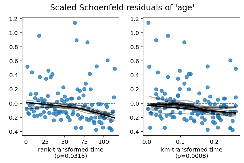
Since age is still violating the proportional hazard assumption, we need to model it better. From the residual plots above, we can see a the effect of age start to become negative over time. This will be relevant later. Below, we present three options to handle age.

Modify the functional form

The proportional hazard test is very sensitive (i.e. lots of false positives) when the functional form of a variable is incorrect. For example, if the association between a covariate and the log-hazard is non-linear, but the model has only a linear term included, then the proportional hazard test can raise a false positive.

The modeller can choose to add quadratic or cubic terms, i.e:

rossi['age**2'] = (rossi['age'] - rossi['age'].mean())**2
rossi['age**3'] = (rossi['age'] - rossi['age'].mean())**3

but I think a more correct way to include non-linear terms is to use basis splines:

cph.fit(rossi, 'week', 'arrest', strata=['wexp'], formula="bs(age, df=4, lower_bound=10, upper_bound=50) + fin +race + mar + paro + prio")
cph.print_summary(model="spline_model"); print()
cph.check_assumptions(rossi, show_plots=True, p_value_threshold=0.05)

model	lifelines.CoxPHFitter
duration col	'week'
event col	'arrest'
strata	[wexp]
baseline estimation	breslow
number of observations	432
number of events observed	114
partial log-likelihood	-579.36
time fit was run	2020-07-26 22:19:25 UTC
model	spline_model

	coef	exp(coef)	se(coef)	coef lower 95%	coef upper 95%	exp(coef) lower 95%	exp(coef) upper 95%	z	p	-log2(p)
covariate
bs(age, df=4, lower_bound=10, upper_bound=50)[0]	-2.95	0.05	8.32	-19.26	13.37	0.00	6.39e+05	-0.35	0.72	0.47
bs(age, df=4, lower_bound=10, upper_bound=50)[1]	-5.48	0.00	6.23	-17.69	6.73	0.00	839.48	-0.88	0.38	1.40
bs(age, df=4, lower_bound=10, upper_bound=50)[2]	-3.69	0.03	8.88	-21.10	13.72	0.00	9.09e+05	-0.42	0.68	0.56
bs(age, df=4, lower_bound=10, upper_bound=50)[3]	-6.02	0.00	6.75	-19.26	7.21	0.00	1351.35	-0.89	0.37	1.43
fin	-0.37	0.69	0.19	-0.75	0.01	0.47	1.01	-1.93	0.05	4.22
race	0.35	1.42	0.31	-0.26	0.95	0.77	2.60	1.13	0.26	1.95
mar	-0.39	0.67	0.38	-1.15	0.36	0.32	1.43	-1.02	0.31	1.71
paro	-0.10	0.90	0.20	-0.49	0.28	0.61	1.33	-0.53	0.60	0.75
prio	0.09	1.10	0.03	0.04	0.15	1.04	1.16	3.22	<0.005	9.59

Concordance	0.62
Partial AIC	1176.72
log-likelihood ratio test	26.82 on 9 df
-log2(p) of ll-ratio test	9.38

Proportional hazard assumption looks okay.

We see may still have potentially some violation, but it’s a heck of a lot less. Also, interestingly, when we include these non-linear terms for age, the wexp proportionality violation disappears. It is not uncommon to see changing the functional form of one variable effects other’s proportional tests, usually positively. So, we could remove the strata=['wexp'] if we wished.

Bin variable and stratify on it

The second option proposed is to bin the variable into equal-sized bins, and stratify like we did with wexp. There is a trade off here between estimation and information-loss. If we have large bins, we will lose information (since different values are now binned together), but we need to estimate less new baseline hazards. On the other hand, with tiny bins, we allow the age data to have the most “wiggle room”, but must compute many baseline hazards each of which has a smaller sample size. Like most things, the optimal value is somewhere inbetween.

rossi_strata_age = rossi.copy()
rossi_strata_age['age_strata'] = pd.cut(rossi_strata_age['age'], np.arange(0, 80, 3))

rossi_strata_age[['age', 'age_strata']].head()

	age	age_strata
0	27	(24, 27]
1	18	(15, 18]
2	19	(18, 21]
3	23	(21, 24]
4	19	(18, 21]

# drop the original, redundant, age column
rossi_strata_age = rossi_strata_age.drop('age', axis=1)
cph.fit(rossi_strata_age, 'week', 'arrest', strata=['age_strata', 'wexp'])

<lifelines.CoxPHFitter: fitted with 432 total observations, 318 right-censored observations>

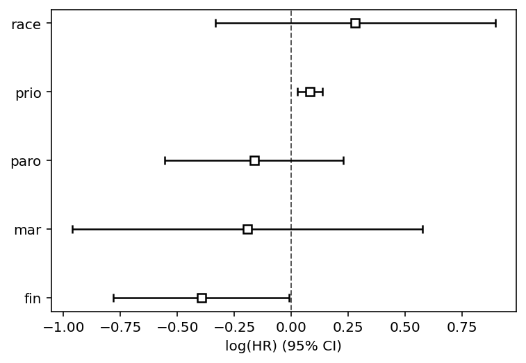
cph.print_summary(3, model="stratified age and wexp")
cph.plot()

model	lifelines.CoxPHFitter
duration col	'week'
event col	'arrest'
strata	[age_strata, wexp]
baseline estimation	breslow
number of observations	432
number of events observed	114
partial log-likelihood	-392.443
time fit was run	2020-07-26 22:19:46 UTC
model	stratified age and wexp

	coef	exp(coef)	se(coef)	coef lower 95%	coef upper 95%	exp(coef) lower 95%	exp(coef) upper 95%	z	p	-log2(p)
covariate
fin	-0.395	0.674	0.197	-0.781	-0.009	0.458	0.991	-2.004	0.045	4.472
race	0.280	1.324	0.313	-0.334	0.895	0.716	2.447	0.895	0.371	1.431
mar	-0.194	0.824	0.392	-0.961	0.574	0.382	1.776	-0.494	0.621	0.687
paro	-0.163	0.849	0.200	-0.555	0.228	0.574	1.256	-0.818	0.413	1.275
prio	0.080	1.084	0.028	0.025	0.135	1.025	1.145	2.854	0.004	7.857

Concordance	0.582
Partial AIC	794.887
log-likelihood ratio test	13.247 on 5 df
-log2(p) of ll-ratio test	5.562

<AxesSubplot:xlabel='log(HR) (95% CI)'>

cph.check_assumptions(rossi_strata_age)

Proportional hazard assumption looks okay.

Introduce time-varying covariates

Our second option to correct variables that violate the proportional hazard assumption is to model the time-varying component directly. This is done in two steps. The first is to transform your dataset into episodic format. This means that we split a subject from a single row into \(n\) new rows, and each new row represents some time period for the subject. It’s okay that the variables are static over this new time periods - we’ll introduce some time-varying covariates later.

See below for how to do this in lifelines:

from lifelines.utils import to_episodic_format

# the time_gaps parameter specifies how large or small you want the periods to be.
rossi_long = to_episodic_format(rossi, duration_col='week', event_col='arrest', time_gaps=1.)
rossi_long.head(25)

	stop	start	arrest	age	fin	id	mar	paro	prio	race	wexp
0	1.0	0.0	0	27	0	0	0	1	3	1	0
1	2.0	1.0	0	27	0	0	0	1	3	1	0
2	3.0	2.0	0	27	0	0	0	1	3	1	0
3	4.0	3.0	0	27	0	0	0	1	3	1	0
4	5.0	4.0	0	27	0	0	0	1	3	1	0
5	6.0	5.0	0	27	0	0	0	1	3	1	0
6	7.0	6.0	0	27	0	0	0	1	3	1	0
7	8.0	7.0	0	27	0	0	0	1	3	1	0
8	9.0	8.0	0	27	0	0	0	1	3	1	0
9	10.0	9.0	0	27	0	0	0	1	3	1	0
10	11.0	10.0	0	27	0	0	0	1	3	1	0
11	12.0	11.0	0	27	0	0	0	1	3	1	0
12	13.0	12.0	0	27	0	0	0	1	3	1	0
13	14.0	13.0	0	27	0	0	0	1	3	1	0
14	15.0	14.0	0	27	0	0	0	1	3	1	0
15	16.0	15.0	0	27	0	0	0	1	3	1	0
16	17.0	16.0	0	27	0	0	0	1	3	1	0
17	18.0	17.0	0	27	0	0	0	1	3	1	0
18	19.0	18.0	0	27	0	0	0	1	3	1	0
19	20.0	19.0	1	27	0	0	0	1	3	1	0
20	1.0	0.0	0	18	0	1	0	1	8	1	0
21	2.0	1.0	0	18	0	1	0	1	8	1	0
22	3.0	2.0	0	18	0	1	0	1	8	1	0
23	4.0	3.0	0	18	0	1	0	1	8	1	0
24	5.0	4.0	0	18	0	1	0	1	8	1	0

Each subject is given a new id (but can be specified as well if already provided in the dataframe). This id is used to track subjects over time. Notice the arrest col is 0 for all periods prior to their (possible) event as well.

Above I mentioned there were two steps to correct age. The first was to convert to a episodic format. The second is to create an interaction term between age and stop. This is a time-varying variable.

Instead of CoxPHFitter, we must use CoxTimeVaryingFitter instead since we are working with a episodic dataset.

rossi_long['time*age'] = rossi_long['age'] * rossi_long['stop']

from lifelines import CoxTimeVaryingFitter
ctv = CoxTimeVaryingFitter()

ctv.fit(rossi_long,
        id_col='id',
        event_col='arrest',
        start_col='start',
        stop_col='stop',
        strata=['wexp'])

<lifelines.CoxTimeVaryingFitter: fitted with 19809 periods, 432 subjects, 114 events>

ctv.print_summary(3, model="age * time interaction")

model	lifelines.CoxTimeVaryingFitter
event col	'arrest'
strata	[wexp]
number of subjects	432
number of periods	19809
number of events	114
partial log-likelihood	-575.080
time fit was run	2020-07-26 22:19:49 UTC
model	age * time interaction

	coef	exp(coef)	se(coef)	coef lower 95%	coef upper 95%	exp(coef) lower 95%	exp(coef) upper 95%	z	p	-log2(p)
covariate
age	0.073	1.075	0.040	-0.005	0.151	0.995	1.163	1.830	0.067	3.893
fin	-0.386	0.680	0.191	-0.760	-0.011	0.468	0.989	-2.018	0.044	4.520
mar	-0.397	0.672	0.382	-1.147	0.352	0.318	1.422	-1.039	0.299	1.743
paro	-0.098	0.907	0.196	-0.481	0.285	0.618	1.330	-0.501	0.616	0.698
prio	0.090	1.094	0.029	0.034	0.146	1.035	1.158	3.152	0.002	9.267
race	0.295	1.343	0.308	-0.310	0.899	0.733	2.458	0.955	0.340	1.558
time*age	-0.005	0.995	0.002	-0.008	-0.002	0.992	0.998	-3.337	0.001	10.203

Partial AIC	1164.160
log-likelihood ratio test	35.386 on 7 df
-log2(p) of ll-ratio test	16.689

ctv.plot()

<AxesSubplot:xlabel='log(HR) (95% CI)'>

In the above scaled Schoenfeld residual plots for age, we can see there is a slight negative effect for higher time values. This is confirmed in the output of the CoxTimeVaryingFitter: we see that the coefficient for time*age is -0.005.

Conclusion

The point estimates and the standard errors are very close to each other using either option, we can feel confident that either approach is okay to proceed.

Do I need to care about the proportional hazard assumption?

You may be surprised that often you don’t need to care about the proportional hazard assumption. There are many reasons why not:

1. If your goal is survival prediction, then you don’t need to care about proportional hazards. Your goal is to maximize some score, irrelevant of how predictions are generated.

2. Given a large enough sample size, even very small violations of proportional hazards will show up.

3. There are legitimate reasons to assume that all datasets will violate the proportional hazards assumption. This is detailed well in Stensrud & Hernán’s “Why Test for Proportional Hazards?” [1].

4. “Even if the hazards were not proportional, altering the model to fit a set of assumptions fundamentally changes the scientific question. As Tukey said,”Better an approximate answer to the exact question, rather than an exact answer to the approximate question.” If you were to fit the Cox model in the presence of non-proportional hazards, what is the net effect? Slightly less power. In fact, you can recover most of that power with robust standard errors (specify robust=True). In this case the interpretation of the (exponentiated) model coefficient is a time-weighted average of the hazard ratio–I do this every single time.” from AdamO, slightly modified to fit lifelines [2]

Given the above considerations, the status quo is still to check for proportional hazards. So if you are avoiding testing for proportional hazards, be sure to understand and able to answer why you are avoiding testing.

1. Stensrud MJ, Hernán MA. Why Test for Proportional Hazards? JAMA. Published online March 13, 2020. doi:10.1001/jama.2020.1267

2. AdamO (https://stats.stackexchange.com/users/8013/adamo), Checking the proportional hazard assumption, URL (version: 2019-04-05): https://stats.stackexchange.com/q/400981