
[1]:
%matplotlib inline
%config InlineBackend.figure_format = 'retina'

from matplotlib import pyplot as plt
from lifelines import CoxPHFitter
import numpy as np
import pandas as pd
from lifelines.datasets import load_rossi

plt.style.use('bmh')
Assessing Cox model fit using residuals (work in progress)
This tutorial is on some common use cases of the (many) residuals of the Cox model. We can use resdiuals to diagnose a model’s poor fit to a dataset, and improve an existing model’s fit.
[2]:
df = load_rossi()

df['age_strata'] = pd.cut(df['age'], np.arange(0, 80, 5))
df = df.drop('age', axis=1)

cph = CoxPHFitter()
cph.fit(df, 'week', 'arrest', strata=['age_strata', 'wexp'])
[2]:
<lifelines.CoxPHFitter: fitted with 432 total observations, 318 right-censored observations>
[3]:
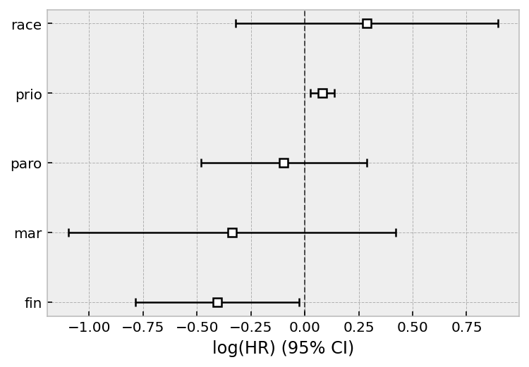
cph.print_summary()
cph.plot();
| model | lifelines.CoxPHFitter |
|---|---|
| duration col | 'week' |
| event col | 'arrest' |
| strata | [age_strata, wexp] |
| baseline estimation | breslow |
| number of observations | 432 |
| number of events observed | 114 |
| partial log-likelihood | -434.50 |
| time fit was run | 2020-07-26 22:06:07 UTC |
| coef | exp(coef) | se(coef) | coef lower 95% | coef upper 95% | exp(coef) lower 95% | exp(coef) upper 95% | z | p | -log2(p) | |
|---|---|---|---|---|---|---|---|---|---|---|
| covariate | ||||||||||
| fin | -0.41 | 0.67 | 0.19 | -0.79 | -0.03 | 0.46 | 0.97 | -2.10 | 0.04 | 4.82 |
| race | 0.29 | 1.33 | 0.31 | -0.32 | 0.90 | 0.73 | 2.45 | 0.93 | 0.35 | 1.50 |
| mar | -0.34 | 0.71 | 0.39 | -1.10 | 0.42 | 0.33 | 1.52 | -0.87 | 0.38 | 1.38 |
| paro | -0.10 | 0.91 | 0.20 | -0.48 | 0.29 | 0.62 | 1.33 | -0.50 | 0.62 | 0.70 |
| prio | 0.08 | 1.08 | 0.03 | 0.02 | 0.14 | 1.03 | 1.15 | 2.83 | <0.005 | 7.73 |
| Concordance | 0.57 |
|---|---|
| Partial AIC | 879.01 |
| log-likelihood ratio test | 13.12 on 5 df |
| -log2(p) of ll-ratio test | 5.49 |
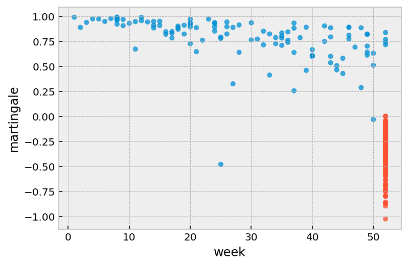
Martingale residuals
Defined as:
where \(T_i\) is the total observation time of subject \(i\) and \(\delta_i\) denotes whether they died under observation of not (event_observed in lifelines).
From [1]:
Martingale residuals take a value between \([1,−\inf]\) for uncensored observations and \([0,−\inf]\) for censored observations. Martingale residuals can be used to assess the true functional form of a particular covariate (Thernau et al. (1990)). It is often useful to overlay a LOESS curve over this plot as they can be noisy in plots with lots of observations. Martingale residuals can also be used to assess outliers in the data set whereby the survivor function predicts an event either too early or too late, however, it’s often better to use the deviance residual for this.
From [2]:
Positive values mean that the patient died sooner than expected (according to the model); negative values mean that the patient lived longer than expected (or were censored).
[4]:
r = cph.compute_residuals(df, 'martingale')
r.head()
/Users/camerondavidson-pilon/code/lifelines/lifelines/utils/__init__.py:924: UserWarning: DataFrame Index is not unique, defaulting to incrementing index instead.
  warnings.warn("DataFrame Index is not unique, defaulting to incrementing index instead.")
[4]:
| week | arrest | martingale | |
|---|---|---|---|
| 313 | 1.0 | True | 0.989383 |
| 79 | 5.0 | True | 0.972812 |
| 60 | 6.0 | True | 0.947726 |
| 225 | 7.0 | True | 0.976976 |
| 138 | 8.0 | True | 0.920272 |
[5]:
r.plot.scatter(
    x='week', y='martingale', c=np.where(r['arrest'], '#008fd5', '#fc4f30'),
    alpha=0.75
)
[5]:
<AxesSubplot:xlabel='week', ylabel='martingale'>
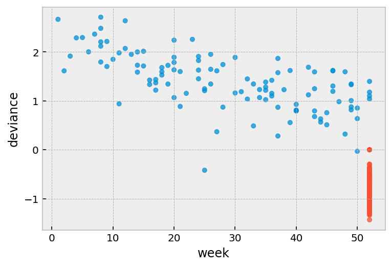
Deviance residuals
One problem with martingale residuals is that they are not symmetric around 0. Deviance residuals are a transform of martingale residuals them symmetric.
Roughly symmetric around zero, with approximate standard deviation equal to 1.
Positive values mean that the patient died sooner than expected.
Negative values mean that the patient lived longer than expected (or were censored).
Very large or small values are likely outliers.
[6]:
r = cph.compute_residuals(df, 'deviance')
r.head()
/Users/camerondavidson-pilon/code/lifelines/lifelines/utils/__init__.py:924: UserWarning: DataFrame Index is not unique, defaulting to incrementing index instead.
  warnings.warn("DataFrame Index is not unique, defaulting to incrementing index instead.")
[6]:
| week | arrest | deviance | |
|---|---|---|---|
| 313 | 1.0 | True | 2.666810 |
| 79 | 5.0 | True | 2.294413 |
| 60 | 6.0 | True | 2.001768 |
| 225 | 7.0 | True | 2.364001 |
| 138 | 8.0 | True | 1.793802 |
[7]:
r.plot.scatter(
    x='week', y='deviance', c=np.where(r['arrest'], '#008fd5', '#fc4f30'),
    alpha=0.75
)
[7]:
<AxesSubplot:xlabel='week', ylabel='deviance'>
[8]:
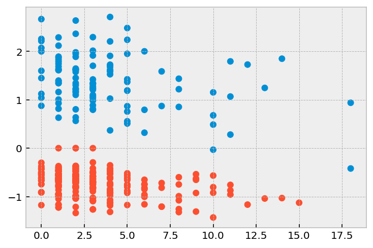
r = r.join(df.drop(['week', 'arrest'], axis=1))
[9]:
plt.scatter(r['prio'], r['deviance'], color=np.where(r['arrest'], '#008fd5', '#fc4f30'))
[9]:
<matplotlib.collections.PathCollection at 0x12a835310>
[ ]:
[10]:
r = cph.compute_residuals(df, 'delta_beta')
r.head()
r = r.join(df[['week', 'arrest']])
r.head()
[10]:
| fin | race | mar | paro | prio | week | arrest | |
|---|---|---|---|---|---|---|---|
| 313 | -0.005650 | -0.011594 | 0.012142 | -0.027450 | -0.020486 | 1 | 1 |
| 79 | -0.005761 | -0.005810 | 0.007687 | -0.020926 | -0.013373 | 5 | 1 |
| 60 | -0.005783 | -0.000147 | 0.003277 | -0.014325 | -0.006315 | 6 | 1 |
| 225 | 0.014998 | -0.041569 | 0.004855 | -0.002254 | -0.015725 | 7 | 1 |
| 138 | 0.011572 | 0.005331 | -0.004240 | 0.013036 | 0.004405 | 8 | 1 |
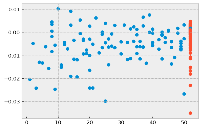
[11]:
plt.scatter(r['week'], r['prio'], color=np.where(r['arrest'], '#008fd5', '#fc4f30'))
[11]:
<matplotlib.collections.PathCollection at 0x11208ab90>
[ ]:
[2] http://myweb.uiowa.edu/pbreheny/7210/f15/notes/11-10.pdf