
Custom regression models
Like for univariate models, it is possible to create your own custom parametric survival models. Why might you want to do this?
Create new / extend AFT models using known probability distributions
Create a piecewise model using domain knowledge about subjects
Iterate and fit a more accurate parametric model
lifelines has a very simple API to create custom parametric regression models. You only need to define the cumulative hazard function. For example, the cumulative hazard for the constant-hazard regression model looks like:
where \(\beta\) are the unknowns we will optimize over.
Below are some example custom models.
[1]:
%matplotlib inline
%config InlineBackend.figure_format = 'retina'

from lifelines.fitters import ParametricRegressionFitter
from autograd import numpy as np
from lifelines.datasets import load_rossi


class ExponentialAFTFitter(ParametricRegressionFitter):

    # this class property is necessary, and should always be a non-empty list of strings.
    _fitted_parameter_names = ['lambda_']

    def _cumulative_hazard(self, params, t, Xs):
        # params is a dictionary that maps unknown parameters to a numpy vector.
        # Xs is a dictionary that maps unknown parameters to a numpy 2d array
        beta = params['lambda_']
        X = Xs['lambda_']
        lambda_ = np.exp(np.dot(X, beta))
        return t / lambda_


rossi = load_rossi()

# the below variables maps {dataframe columns, formulas} to parameters
regressors = {
    # could also be: 'lambda_': rossi.columns.difference(['week', 'arrest'])
    'lambda_': "age + fin + mar + paro + prio + race + wexp + 1"
}

eaf = ExponentialAFTFitter().fit(rossi, 'week', 'arrest', regressors=regressors)
eaf.print_summary()
| model | lifelines.ExponentialAFTFitter |
|---|---|
| duration col | 'week' |
| event col | 'arrest' |
| number of observations | 432 |
| number of events observed | 114 |
| log-likelihood | -686.37 |
| time fit was run | 2020-07-26 22:06:42 UTC |
| coef | exp(coef) | se(coef) | coef lower 95% | coef upper 95% | exp(coef) lower 95% | exp(coef) upper 95% | z | p | -log2(p) | ||
|---|---|---|---|---|---|---|---|---|---|---|---|
| param | covariate | ||||||||||
| lambda_ | Intercept | 4.05 | 57.44 | 0.59 | 2.90 | 5.20 | 18.21 | 181.15 | 6.91 | <0.005 | 37.61 |
| age | 0.06 | 1.06 | 0.02 | 0.01 | 0.10 | 1.01 | 1.10 | 2.55 | 0.01 | 6.52 | |
| fin | 0.37 | 1.44 | 0.19 | -0.01 | 0.74 | 0.99 | 2.10 | 1.92 | 0.06 | 4.18 | |
| mar | 0.43 | 1.53 | 0.38 | -0.32 | 1.17 | 0.73 | 3.24 | 1.12 | 0.26 | 1.93 | |
| paro | 0.08 | 1.09 | 0.20 | -0.30 | 0.47 | 0.74 | 1.59 | 0.42 | 0.67 | 0.57 | |
| prio | -0.09 | 0.92 | 0.03 | -0.14 | -0.03 | 0.87 | 0.97 | -3.03 | <0.005 | 8.65 | |
| race | -0.30 | 0.74 | 0.31 | -0.91 | 0.30 | 0.40 | 1.35 | -0.99 | 0.32 | 1.63 | |
| wexp | 0.15 | 1.16 | 0.21 | -0.27 | 0.56 | 0.76 | 1.75 | 0.69 | 0.49 | 1.03 |
| AIC | 1388.73 |
|---|---|
| log-likelihood ratio test | 31.22 on 7 df |
| -log2(p) of ll-ratio test | 14.11 |
[2]:
class DependentCompetingRisksHazard(ParametricRegressionFitter):
"""
Reference
--------------
Frees and Valdez, UNDERSTANDING RELATIONSHIPS USING COPULAS
"""
_fitted_parameter_names = ["lambda1", "rho1", "lambda2", "rho2", "alpha"]
def _cumulative_hazard(self, params, T, Xs):
lambda1 = np.exp(np.dot(Xs["lambda1"], params["lambda1"]))
lambda2 = np.exp(np.dot(Xs["lambda2"], params["lambda2"]))
rho2 = np.exp(np.dot(Xs["rho2"], params["rho2"]))
rho1 = np.exp(np.dot(Xs["rho1"], params["rho1"]))
alpha = np.exp(np.dot(Xs["alpha"], params["alpha"]))
return ((T / lambda1) ** rho1 + (T / lambda2) ** rho2) ** alpha
fitter = DependentCompetingRisksHazard(penalizer=0.1)
rossi = load_rossi()
rossi["week"] = rossi["week"] / rossi["week"].max() # scaling often helps with convergence
covariates = {
"lambda1": rossi.columns.difference(['week', 'arrest']),
"lambda2": rossi.columns.difference(['week', 'arrest']),
"rho1": "1",
"rho2": "1",
"alpha": "1",
}
fitter.fit(rossi, "week", event_col="arrest", regressors=covariates, timeline=np.linspace(0, 2))
fitter.print_summary(2)
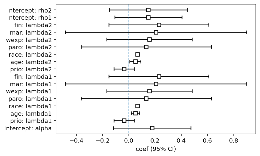
ax = fitter.plot()
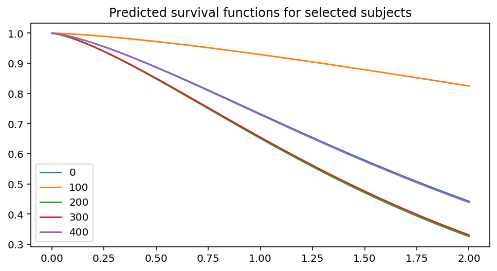
ax = fitter.predict_survival_function(rossi.loc[::100]).plot(figsize=(8, 4))
ax.set_title("Predicted survival functions for selected subjects")
/Users/camerondavidson-pilon/code/lifelines/lifelines/fitters/__init__.py:1985: StatisticalWarning: The diagonal of the variance_matrix_ has negative values. This could be a problem with DependentCompetingRisksHazard's fit to the data.

It's advisable to not trust the variances reported, and to be suspicious of the fitted parameters too.

  warnings.warn(warning_text, exceptions.StatisticalWarning)
| model | lifelines.DependentCompetingRisksHazard |
|---|---|
| duration col | 'week' |
| event col | 'arrest' |
| penalizer | 0.1 |
| number of observations | 432 |
| number of events observed | 114 |
| log-likelihood | -239.19 |
| time fit was run | 2020-07-26 22:06:55 UTC |
| coef | exp(coef) | se(coef) | coef lower 95% | coef upper 95% | exp(coef) lower 95% | exp(coef) upper 95% | z | p | -log2(p) | ||
|---|---|---|---|---|---|---|---|---|---|---|---|
| param | covariate | ||||||||||
| lambda1 | age | 0.05 | 1.05 | 0.02 | 0.02 | 0.08 | 1.02 | 1.09 | 3.06 | <0.005 | 8.80 |
| fin | 0.23 | 1.26 | 0.19 | -0.15 | 0.61 | 0.86 | 1.84 | 1.18 | 0.24 | 2.06 | |
| mar | 0.21 | 1.23 | 0.35 | -0.48 | 0.90 | 0.62 | 2.46 | 0.59 | 0.56 | 0.84 | |
| paro | 0.13 | 1.14 | 0.25 | -0.36 | 0.63 | 0.69 | 1.88 | 0.52 | 0.60 | 0.74 | |
| prio | -0.04 | 0.96 | 0.04 | -0.11 | 0.04 | 0.89 | 1.04 | -0.93 | 0.35 | 1.50 | |
| race | 0.07 | 1.07 | nan | nan | nan | nan | nan | nan | nan | nan | |
| wexp | 0.16 | 1.17 | 0.17 | -0.17 | 0.48 | 0.85 | 1.62 | 0.94 | 0.35 | 1.53 | |
| lambda2 | age | 0.05 | 1.05 | 0.02 | 0.01 | 0.09 | 1.01 | 1.10 | 2.34 | 0.02 | 5.70 |
| fin | 0.23 | 1.26 | 0.19 | -0.15 | 0.61 | 0.86 | 1.84 | 1.18 | 0.24 | 2.06 | |
| mar | 0.21 | 1.23 | 0.35 | -0.48 | 0.90 | 0.62 | 2.46 | 0.59 | 0.56 | 0.84 | |
| paro | 0.13 | 1.14 | 0.25 | -0.36 | 0.63 | 0.69 | 1.88 | 0.52 | 0.60 | 0.74 | |
| prio | -0.04 | 0.96 | 0.04 | -0.11 | 0.04 | 0.89 | 1.04 | -0.93 | 0.35 | 1.50 | |
| race | 0.07 | 1.07 | nan | nan | nan | nan | nan | nan | nan | nan | |
| wexp | 0.16 | 1.17 | 0.17 | -0.17 | 0.48 | 0.85 | 1.62 | 0.94 | 0.35 | 1.53 | |
| rho1 | Intercept | 0.15 | 1.16 | 0.13 | -0.11 | 0.40 | 0.90 | 1.50 | 1.14 | 0.25 | 1.98 |
| rho2 | Intercept | 0.15 | 1.16 | 0.15 | -0.15 | 0.44 | 0.86 | 1.56 | 0.99 | 0.32 | 1.62 |
| alpha | Intercept | 0.18 | 1.19 | 0.15 | -0.12 | 0.47 | 0.89 | 1.61 | 1.18 | 0.24 | 2.06 |
| AIC | 512.38 |
|---|---|
| log-likelihood ratio test | 127.04 on 12 df |
| -log2(p) of ll-ratio test | 68.48 |
[2]:
Text(0.5, 1.0, 'Predicted survival functions for selected subjects')
Cure models
Suppose in our population we have a subpopulation that will never experience the event of interest. Or, for some subjects the event will occur so far in the future that it’s essentially at time infinity. In this case, the survival function for an individual should not asymptically approach zero, but some positive value. Models that describe this are sometimes called cure models (i.e. the subject is “cured” of death and hence no longer susceptible) or time-lagged conversion models.
It would be nice to be able to use common survival models and have some “cure” component. Let’s suppose that for individuals that will experience the event of interest, their survival distribution is a Weibull, denoted \(S_W(t)\). For a random selected individual in the population, their survival curve, \(S(t)\), is:
Even though it’s in an unconventional form, we can still determine the cumulative hazard (which is the negative logarithm of the survival function):
[3]:
from autograd.scipy.special import expit

class CureModel(ParametricRegressionFitter):
    _scipy_fit_method = "SLSQP"
    _scipy_fit_options = {"ftol": 1e-10, "maxiter": 200}

    _fitted_parameter_names = ["lambda_", "beta_", "rho_"]

    def _cumulative_hazard(self, params, T, Xs):
        c = expit(np.dot(Xs["beta_"], params["beta_"]))

        lambda_ = np.exp(np.dot(Xs["lambda_"], params["lambda_"]))
        rho_ = np.exp(np.dot(Xs["rho_"], params["rho_"]))
        sf = np.exp(-(T / lambda_) ** rho_)

        return -np.log((1 - c) + c * sf)


cm = CureModel(penalizer=0.0)

rossi = load_rossi()

covariates = {"lambda_": rossi.columns.difference(['week', 'arrest']), "rho_": "1", "beta_": 'fin + 1'}

cm.fit(rossi, "week", event_col="arrest", regressors=covariates, timeline=np.arange(250))
cm.print_summary(2)
| model | lifelines.CureModel |
|---|---|
| duration col | 'week' |
| event col | 'arrest' |
| number of observations | 432 |
| number of events observed | 114 |
| log-likelihood | -702.64 |
| time fit was run | 2020-07-26 22:07:13 UTC |
| coef | exp(coef) | se(coef) | coef lower 95% | coef upper 95% | exp(coef) lower 95% | exp(coef) upper 95% | z | p | -log2(p) | ||
|---|---|---|---|---|---|---|---|---|---|---|---|
| param | covariate | ||||||||||
| lambda_ | age | 0.16 | 1.17 | 0.05 | 0.05 | 0.26 | 1.06 | 1.30 | 2.96 | <0.005 | 8.36 |
| fin | 1.14 | 3.13 | 4320.37 | -8466.63 | 8468.92 | 0.00 | inf | 0.00 | 1.00 | 0.00 | |
| mar | 0.35 | 1.42 | 0.32 | -0.27 | 0.97 | 0.76 | 2.64 | 1.11 | 0.27 | 1.90 | |
| paro | 0.26 | 1.30 | 0.24 | -0.20 | 0.72 | 0.82 | 2.06 | 1.10 | 0.27 | 1.88 | |
| prio | -0.02 | 0.98 | 0.04 | -0.10 | 0.06 | 0.91 | 1.06 | -0.51 | 0.61 | 0.71 | |
| race | 0.23 | 1.26 | 0.28 | -0.32 | 0.79 | 0.72 | 2.20 | 0.82 | 0.41 | 1.29 | |
| wexp | 0.25 | 1.28 | 0.17 | -0.08 | 0.57 | 0.92 | 1.78 | 1.49 | 0.14 | 2.86 | |
| rho_ | Intercept | 0.13 | 1.14 | 0.08 | -0.03 | 0.29 | 0.97 | 1.34 | 1.57 | 0.12 | 3.11 |
| beta_ | Intercept | 0.18 | 1.19 | 0.10 | -0.02 | 0.37 | 0.98 | 1.45 | 1.75 | 0.08 | 3.64 |
| fin | 15.80 | 7.30e+06 | 0.17 | 15.46 | 16.14 | 5.20e+06 | 1.03e+07 | 90.99 | <0.005 | inf |
| AIC | 1425.29 |
|---|---|
| log-likelihood ratio test | -12.04 on 7 df |
| -log2(p) of ll-ratio test | -0.00 |
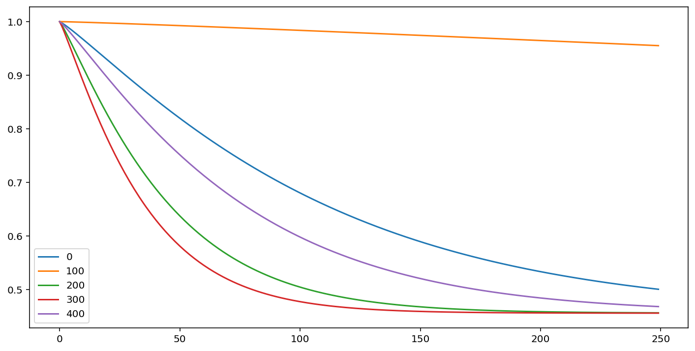
[4]:
cm.predict_survival_function(rossi.loc[::100]).plot(figsize=(12,6))
[4]:
<AxesSubplot:>
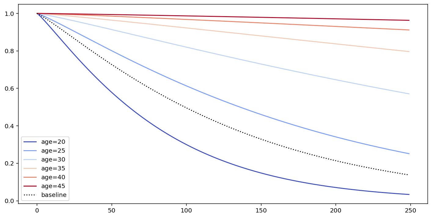
[5]:
# what's the effect on the survival curve if I vary "age"
fig, ax = plt.subplots(figsize=(12, 6))

cm.plot_covariate_groups(['age'], values=np.arange(20, 50, 5), cmap='coolwarm', ax=ax)
[5]:
<AxesSubplot:>
Spline models
See royston_parmar_splines.py in the examples folder: https://github.com/CamDavidsonPilon/lifelines/tree/master/examples